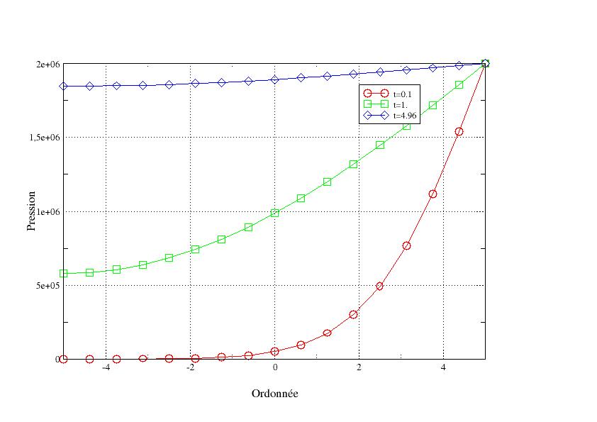
Illustration 1: Pression sur le bord droit à 3 instants
v7.32.129 WTNP129 – Modélisation HM d’un barreau saturé en liquide compressible#
Résumé:
On étudie ici un problème HM saturé en liquide en dimension 2. Vu les symétries du problème traité, la solution est unidimensionnelle. La structure est soumise à une pression hydraulique imposée sur sa partie supérieure. Son comportement mécanique est élastique. Ce test a pour but de tester la résolution par couplage (cf documentation «Notice d’utilisation du modèle THM» [U2.04.05])
On a donc 3 modélisations dans ce test :
Modélisation A : on résout le problème physique à l’aide de la méthode «classique», par couplage global
Modélisation C : Cette modélisation est identique à la modélisation A mais avec l’élément sous-intégré HM_SI
Solution de référence#
On s’intéresse aux valeurs de DY, PRE1 et SIYY en 5 nœuds (\(\mathrm{N4}\) , \(\mathrm{N23}\) , \(\mathrm{N27}\) , \(\mathrm{N31}\) , \(\mathrm{N1}\) ) situés sur le bord droit du barreau aux deux instants \(t=1\) sec et \(t=10\) secondes.
Les tests effectués sont des tests de non-régression pour la modélisation A.
Pour la modélisation C, les tests effectués sont des tests d’adhérence aux résultats de la modélisation A (de type AUTRE_ASTER).
Modélisation A#
Caractéristiques de la modélisation#
On utilise la modélisation D_PLAN_HMS.
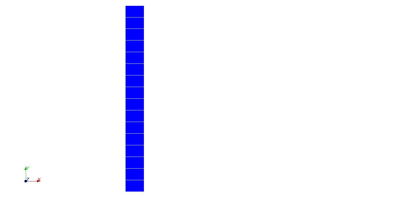
Caractéristiques du maillage#
Nombre de nœuds: 83
Nombre de mailles et types: 16 mailles QUAD8
Grandeurs testées et résultats#
On réalise les tests de non-régression suivants.
Identification |
Type de référence |
Référence |
\(\mathrm{N23}\) – PRE1- \(t=1\) |
NON_REGRESSION |
1.4477057505633E+06 |
\(\mathrm{N27}\) – PRE1- \(t=1\) |
NON_REGRESSION |
9.8618261792096E+05 |
\(\mathrm{N31}\) – PRE1- \(t=1\) |
NON_REGRESSION |
6.8416253970115E+05 |
\(\mathrm{N1}\) – PRE1- \(t=1\) |
NON_REGRESSION |
5.7968660741362E+05 |
\(\mathrm{N23}\) – PRE1- \(t=10\) |
NON_REGRESSION |
1.9965914222579E+06 |
\(\mathrm{N27}\) – PRE1- \(t=10\) |
NON_REGRESSION |
1.9937017653319E+06 |
\(\mathrm{N31}\) – PRE1- \(t=10\) |
NON_REGRESSION |
1.9917709562082E+06 |
\(\mathrm{N1}\) – PRE1- \(t=10\) |
NON_REGRESSION |
1.991092945817E+06 |
\(\mathrm{N4}\) – DY- \(t=1\) |
NON_REGRESSION |
1.8807606329922E-03 |
\(\mathrm{N23}\) – DY- \(t=1\) |
NON_REGRESSION |
1.139326750168E-03 |
\(\mathrm{N27}\) – DY- \(t=1\) |
NON_REGRESSION |
6.19182033214E-04 |
\(\mathrm{N31}\) – DY- \(t=1\) |
NON_REGRESSION |
2.6539252530741E-04 |
\(\mathrm{N4}\) – DY- \(t=10\) |
NON_REGRESSION |
3.4385071565836E-03 |
\(\mathrm{N23}\) – DY- \(t=10\) |
NON_REGRESSION |
2.5771817886894E-03 |
\(\mathrm{N27}\) – DY- \(t=10\) |
NON_REGRESSION |
1.7172304114012E-03 |
\(\mathrm{N31}\) – DY- \(t=10\) |
NON_REGRESSION |
8.5833064233171E-04 |
\(\mathrm{N4}\) – SIYY- \(t=1\) |
NON_REGRESSION |
2.00000E+06 |
\(\mathrm{N23}\) – SIYY- \(t=1\) |
NON_REGRESSION |
1.4477057505633E+06 |
\(\mathrm{N27}\) – SIYY- \(t=1\) |
NON_REGRESSION |
9.8618261792096E+05 |
\(\mathrm{N31}\) – SIYY- \(t=1\) |
NON_REGRESSION |
6.8416253970115E+05 |
\(\mathrm{N1}\) – SIYY- \(t=1\) |
NON_REGRESSION |
5.7968660741362E+05 |
\(\mathrm{N4}\) – SIYY- \(t=10\) |
NON_REGRESSION |
2.00000E+06 |
\(\mathrm{N23}\) – SIYY- \(t=10\) |
NON_REGRESSION |
1.9965914222579E+06 |
\(\mathrm{N27}\) – SIYY- \(t=10\) |
NON_REGRESSION |
1.9937017653319E+06 |
\(\mathrm{N31}\) – SIYY- \(t=10\) |
NON_REGRESSION |
1.9917709562082E+06 |
\(\mathrm{N1}\) – SIYY- \(t=10\) |
NON_REGRESSION |
1.991092945817E+06 |
Modélisation C#
Caractéristiques de la modélisation#
On utilise la modélisation D_PLAN_HM_SI.
Caractéristiques du maillage#
Nombre de nœuds: 83
Nombre de mailles et types: 16 mailles QUAD8
Grandeurs testées et résultats#
Les tests de non-régression sont effectués en version 11.0.25.
Identification |
Type de référence |
Référence |
Erreur |
\(\mathrm{N23}\) – PRE1- \(t=1\) |
AUTRE_ASTER |
1.4477057505633E+06 |
0.0044% |
\(\mathrm{N27}\) – PRE1- \(t=1\) |
AUTRE_ASTER |
9.8618261792096E+05 |
0.0462% |
\(\mathrm{N31}\) – PRE1- \(t=1\) |
AUTRE_ASTER |
6.8416253970115E+05 |
0.151% |
\(\mathrm{N1}\) – PRE1- \(t=1\) |
AUTRE_ASTER |
5.7968660741362E+05 |
0.226% |
\(\mathrm{N4}\) – DY- \(t=1\) |
AUTRE_ASTER |
1.8807606329922E-03 |
0.0506% |
\(\mathrm{N23}\) – DY- \(t=1\) |
AUTRE_ASTER |
1.139326750168E-03 |
0.0829% |
\(\mathrm{N27}\) – DY- \(t=1\) |
AUTRE_ASTER |
6.19182033214E-04 |
0.136% |
\(\mathrm{N31}\) – DY- \(t=1\) |
AUTRE_ASTER |
2.6539252530741E-04 |
0.197% |
\(\mathrm{N4}\) – SIYY- \(t=1\) |
AUTRE_ASTER |
2.00000E+06 |
1.0E-13% |
\(\mathrm{N23}\) – SIYY- \(t=1\) |
AUTRE_ASTER |
1.4477057505633E+06 |
0.0044% |
\(\mathrm{N27}\) – SIYY- \(t=1\) |
AUTRE_ASTER |
9.8618261792096E+05 |
0.0462% |
\(\mathrm{N31}\) – SIYY- \(t=1\) |
AUTRE_ASTER |
6.8416253970115E+05 |
0.151% |
\(\mathrm{N1}\) – SIYY- \(t=1\) |
AUTRE_ASTER |
5.7968660741362E+05 |
0.226% |
\(\mathrm{N23}\) – PRE1- \(t=10\) |
AUTRE_ASTER |
1.9965914222579E+06 |
0.0012% |
\(\mathrm{N27}\) – PRE1- \(t=10\) |
AUTRE_ASTER |
1.9937017653319E+06 |
0.0023% |
\(\mathrm{N31}\) – PRE1- \(t=10\) |
AUTRE_ASTER |
1.9917709562082E+06 |
0.003% |
\(\mathit{N1}\) – PRE1- \(t=10\) |
AUTRE_ASTER |
1.991092945817E+06 |
0.0032% |
\(\mathit{N4}\) – DY- \(t=10\) |
AUTRE_ASTER |
3.4385071565836E-03 |
0.002% |
\(\mathit{N23}\) – DY- \(t=10\) |
AUTRE_ASTER |
2.5771817886894E-03 |
0.0025% |
\(\mathit{N27}\) – DY- \(t=10\) |
AUTRE_ASTER |
1.7172304114012E-03 |
0.0029% |
\(\mathit{N31}\) – DY- \(t=10\) |
AUTRE_ASTER |
8.5833064233171E-04 |
0.0031% |
\(\mathit{N4}\) – SIYY- \(t=10\) |
AUTRE_ASTER |
2.00000E+06 |
1E-13% |
\(\mathit{N23}\) – SIYY- \(t=10\) |
AUTRE_ASTER |
1.9965914222579E+06 |
0.0012% |
\(\mathit{N27}\) – SIYY- \(t=10\) |
AUTRE_ASTER |
1.9937017653319E+06 |
0.0023% |
\(\mathit{N31}\) – SIYY- \(t=10\) |
AUTRE_ASTER |
1.9917709562082E+06 |
0.003% |
\(\mathit{N1}\) – SIYY- \(t=10\) |
AUTRE_ASTER |
1.991092945817E+06 |
0.0032% |
Synthèse des résultats#
Les valeurs fournies par Code_Aster sont en parfait accord avec les valeurs de référence.