r7.02.22 Calculation of modified J-integral in presence of initial state#

Summary:

This document aims at describing the theoretical formulations and implementation to compute the modified J -integral in 3D and 2D via the macro_command POST_JMOD.

The theoretical background of J -integral is presented in Section 1 . It is first introduced by the continuous mathematical description of the standard J in 2D [1]. This standard formulation without initial state is extended successively to the full 3D formulation [2] and the modified formulations to account for the presence of an initial strain field [3] and the non-proportional loading conditions [4]. In Section 2 , the domain integral formulations are detailed in discretized form adapted for the finite element method. The overall strategy for implementation of the macro_command POST_JMOD in code_aster , and general information regarding the supported element types, loads, and required mechanics fields are presented in Section 3 . Specific details of the procedures used in the identification of key terms such as the virtual crack extension field, the cracked surface advancement and the gradient of the deformation and strain energy terms are presented in Section 2 . Finally, an overview list of the test cases used to validate POST_JMOD is presented in Section 3 .

The current development version of POST_JMOD is applicable for:

elastic and plastic material behaviors;
proportional/non-proportional and mixed mode loads;
initial strain (associated with an equilibrium residual stress);
Standard FEM with a meshed crack

Table of Contents

Table of Figures

Discretized formulation implemented within POST_JMOD#

The domain integral formulations presented in Section 1 are conveniently implemented in discretized form. The general equations of modified J -integral without and with presence of initial strain Equation 9 and Equation 10 are re-written here by the finite element method.

The first, the global coordinates xi may be written as:

… (14)

where ne is the number of nodes per element, Nk are the shape functions and Xik are the nodal coordinates.

The nodal fields describing the displacements ui , the qi fields and the initial strain ε0 are written in a similar way:

where Uik are the nodal displacements, Qik are the nodal values of virtual crack extension, and εijk0 are the nodal values of initial strain.

It is noted that the strain ε and the energy W are evaluated at Gauss points. For calculating their gradients, these fields are first converted to global nodal fields (XXXX_ELGA to XXXX_NOEU in code_aster ). This conversion introduces an approximation error due to the fact that a simple arithmetic mean (with no consideration of mesh size) of the connected nodes is used to evaluate the global nodal values. However, this approximation allows us to avoid the issue that locally the strain gradients are null on the element, when considering classical finite element methods.

The gradients of these fields are given by:

\(\frac{{\partial \epsilon }_{ij}}{{\partial x}_{n}}\approx \sum_{k=1}^{\mathit{ng}}\sum_{l=1}^{3}\frac{{\partial N}_{k}}{\partial {\eta}_{l}}\frac{\partial {\eta}_{l}}{{\partial N}_{k}}{{\epsilon}_{\mathit{ijk}}|}_{\mathit{NOEU}}\) (21)

\(\frac{\partial W}{{\partial x}_{n}}\approx \sum_{k=1}^{\mathit{ng}}\sum_{l=1}^{3}\frac{{\partial N}_{k}}{\partial {\eta}_{l}}\frac{\partial {\eta}_{l}}{{\partial N}_{k}}{{W}_{k}|}_{\mathit{NOEU}}\) (22)

where ηl represents the local coordinates ( η1, η2, η3 ) and ∂ ηl /∂ xm is the inverse Jacobian matrix of the transformation in Equation 14, and the terms with | NOEU Indicate that the global nodal values have been used in the computation, which were obtained from Gaussian values as described earlier.

The domain integral expression of modified J without initial stress in Equation Error: Reference source not found is:

where nV represents the number of elements in the volume V , nV1 represents the number of elements in the volume V1 and ng is the number of gauss points per element. The quantities within {.} p are evaluated at all Gauss points in an element and wp are the respective weights.

The domain integral expression of modified J with initial stress in Equation 10 is:

In the development of POST_JMOD, the Equations 23-24 are calculated using POST_ELEM operator.

Algorithm of POST_JMOD J-integral in code_aster#

Approach to compute fracture mechanics parameters in presence of initial strain#

There are three main steps in the computation of fracture mechanics parameters in the presence of initial state:

Create a field at the initial state

There are two types of initial state: the first is a result field from a computation step (as described in section 1.5) and the second ay result from importing an external residual stress/strain field.. It is important to verify that the initial state is in auto-equilibrium. For example, from an initial stress field, one can deduce an equivalent initial strains field. By performing a dummy step with no applied loads, one can verify if the initial state is in auto-equilibrium. The user must be aware that the fields given to POST_JMOD are appropriate.

Perform a mechanics computation including initial state for a cracked structure
Post-processing using POST_JMOD

STEP 1 : Create an initial state Using STAT_NON_LINE or by CREA_CHAMP If using CREA_CHAMP, verify that the initial stress is in auto-equilibrium
STEP 2 : Mechanical calculation with initial stress and cracked structure
SIG_0 ≠ 0+ CRACK	→ (STAT_NON_LINE) →	SIG≠ 0, EPS≠ 0
STEP 3 : J calculation in presence of initial state
POST_JMOD=(… ETAT_INIT=_F(EPSI=EPS_0)

Figure 7- Steps in computation of fracture mechanics

Steps in strategy implementation#

POST_JMOD is developed as a python based macro command in order to execure step 3 of Figure 7. The programmed algorithm is contained within POST_JMOD_ops.py. The script contains all the necessary functions in order to perform the calculation described within Section 2 . However, some minor changes to the FOTRAN90 code were made in order to enable computation for large numbers of contours. This is a simple change to the size of the number of nodes defined by INFNORM_NOEU2 within defi_fond_fiss.

The general sequence of computation is described by the following diagram:

Firstly, using in built operators, the mesh geometrical data, model is extracted and the field results containing the global displacement field at node points and stress, strain, energy fields at gauss points. This represents the raw information used to setup the algorithm and computation. An example of the syntax used is given:

MAIL = self.getModel().getMesh()

MODE = self.getModel()

__RESU = RESULTAT

__RESU = CALC_CHAMP(reuse=__RESU,

RESULTAT=__RESU,

CONTRAINTE=(“SIGM_ELGA”),

DEFORMATION=(“EPSI_ELGA”),

ENERGIE=(“ETOT_ELGA”),)

Secondly, from the data structure of the crack defined by DEFI_FOND_FISS, information regarding the crack is extracted: element type, the presence of symmetry, opened/closed crack type, crack surfaces. This information is used for determining number of nodes on the crack front, set of nodes on the crack surfaces through nodes of crack front. The information is also used to create logic gates within the POST_JMOD_ops.py files in order to correctly apply the computation as data structures are different sizes and types.

elemType = FOND_FISS.getCrackTipCellsType()

ir, ib, symeType = aster.dismoi(“SYME”,FOND_FISS.getName(),”FOND_FISS”, “F”)

NP, TPFISS, closedCrack = no_fond_fiss(self, FOND_FISS)

Then, the virtual crack extension field is computed. This field is substitute as the q field in the J -integral computation. Further details of this step are given in Section 2.1
Next, the volume domain V for the calculation is identified according to user specified number of contours. Once the integral volume is determined, all nodes are extracted from this volume and the q fields are assigned to these nodes. In this development, the number of contours must be greater than or equal to 2. Details of this step are given in Section 2.2 and 2.3 .
Then, the virtual area increase of the cracked surface generated by application of virtual crack extension is calculated. To do this, the nodes on the crack surface are translated according to the virtual crack extension vectors to compute the area. Note that this is only performed to calculate the area increase and the mesh remains unchanged for the J-Integral computation. Further details of this step are given in Section 2.4 .
Next, following the problem as linear/non-linear problem, the J -integral is calculated at each instant of calculation and at each node of crack front. The calculated fields such as virtual crack extension q , stress, strain, displacement, energy, and their gradients/divergence can be extracted from the results or can be computed using CREA_CHAMP, CREA_RESU, and CALC_CHAMP operators. The non-conventional terms are detailed in Section 2.5 and Section 2.6 .

Here is a pseudo-code for the loops on instants and on nodes and the calculation/combination of terms:

Q_FIELD

for INST in LIST_INST:

STRESS_FIELD

DISPLACEMENT_FIELD

GRAD_OF_DISPLACEMENT_FIELD

STRAIN_FIELD

GRAD_OF_STRAIN_FIELD

if presence_of_initial_strain:

INITIAL_STRAIN_FIELD

GRAD_OF_INITIAL_STRAIN_FIELD

STRAIN_ENERGY_FIELD

GRAD_OF_STRAIN_ENERGY_FIELD

for INODE in LIST_NODE:

GRAD_OF_Q_FIELD

COMPUTE EACH TERME OF EQUATIONS Error: Reference source not found AND Error: Reference source not found IN SECTION 2

J=COMBINATION OF TERMES

At the end of POST_JMOD macro_command, the results of J are printed under format table of code_aster using CREA_TABLE and CALC_TABLE.

Restrictions on Element types and loads#

The J -integral may be applied to a 3D problem where it is defined locally around the crack tip points along the crack front in the planes perpendicular to the crack front (see Figure 2 ), as discussed in section 1. The procedure to calculate J has only been developed with hexahedral elements in mind. However, for complex 3D cracks, it is possible to use the prism elements for the first ring around the crack front. It must be noted that one of the quadrangle surfaces of these prism elements should be located on one of the crack surfaces ( Figure 8 ). This restriction comes from the difficulty in determination of crack propagation direction and of the area increase of the cracked surface with irregular meshes. The user must take to ensure an appropriate mesh is utilised in the computation.

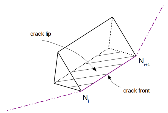
Figure 8: Definition of the pentahedral element for J calculation.

It should be emphasized that the same limit was observed in the J -integral development of Abaqus software [7]: “ The contour integral evaluation capability of ABAQUS assumes that the elements that lie within the domain used for the calculations are quadrilaterals in two-dimensional or shell models or bricks in continuum three-dimensional models. Triangles, tetrahedrals, or wedges should not be used in the mesh that is included in the contour integral regions ”.

In code_aster , it is possible to calculate the J -integral using the command POST_JMOD [U4.82.41]. The virtual crack extension field of the crack q is calculated automatically in this command from the information provided by the user. The current development is valid for the 3D modeling and deals with the following conditions only:

both elastic and plastic behaviors of materials;
proportional, non-proportional and mixed mode loads;
initial strains (representing residual stress fields)

It cannot deal with cases where there is pressure on the crack surfaces.

Required existing code_aster concepts#

For the calculation of the energy release rate, it is necessary to characterize beforehand the meshed crack via the concept of the FOND_FISS type with the command DEFI_FOND_FISS [U4.82.01]. The current version of POST_JMOD has not been yet available for non-meshed (X-FEM) crack. As discussed later, hexahedral elements need to be used in the regions around the crack tip which are used to compute domain integral.

Developments specific to POST_JMOD formulation#

Computation of virtual crack extension field q#

In this section, we show how to determine the virtual crack extension field q which is defined by Equation 3 at each node point of crack front when the crack front is defined by straight segments and the crack surface is defined by flat element faces. The vector q is defined here on all the nodes within volume integration limited by number of contours and not on a line, and q=0 for all nodes on boundary. Then, the integral is evaluated on this volume. In this development, the q value calculated by Equation 30 is used for assigning (this is not case that was done in 2D by Lei).

We consider a crack fissure with crack front on which the node Ni and its neighbors Ni-1, Ni+1 are presented and its surface ( Figure 9 ). We will determine **qi* at node Ni.

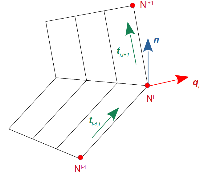
Figure 9: A crack with crack front and its surface.

First, two vectors **ti-1,i* and **ti,i+1* along two neighboring segments of the crack front are determined:

where **ui-1* , **ui* , **ui+1* are coordinates of Ni-1, Ni, Ni+1, respectively, and ||.|| denotes vector length.

The virtual crack extension **qi* at the crack front node Ni is obtained by averaging the two following vectors:

where n is a normalized vector of crack surface at node Ni and can be determined as:

Finally, the virtual crack extension q is calculated as:

Extension of contour domain identification from 2D to 3D#

In this section, the methods to identify the domain integral in 2D and 3D are discussed.

For a 2D meshed crack, an example of two contours around crack tip N are shown in Figure 10 . As shown in the figure, the contours are made to coincide with the edges of the elements, the q fields are assigned on the nodes of these contours and the J-integral is evaluated on the 2D surface area enclosed by each contour.

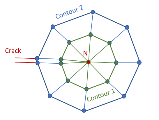
Figure 10: The defined contours around crack tip in 2D problem.

In 3D problems, in order to illustrate the extension, we first assume that for each node along the crack front, there exists a plane perpendicular to the crack front through this node ( Figure 11 ), e.g. plane (Pi) through node Ni. On each plane, the contour is identified in the same manner as the 2D case for two successive planes as shown in Figure 12 . These nodes become the two surfaces of the torus along the NiNi+1 direction. The contours are made of the surfaces of the elements, the q fields are assigned on the nodes of these contours and the integral is evaluated on the volume 3D .

As mentioned in Section 1.3 , in 3 D , hexahedral meshes are used in the contour integral regions and it is possible to use the pentahedral elements for the first ring around the crack front. This allows the existence of a plane that passes each node of crack front.

When considering the discretised problem by the finite element method, we note that it is possible that the set of nodes defining the contours that for each nodal position along the crack front may not all lie on a single mathematical plane, as the assumed theory of J -integrals in 3D discussed earlier. However, they are well defined on a single surface. Note that a surface here is defined as a group of element surfaces and they do not necessarily all lie on a plane. More specifically, the left hand image in Figure 13 shows the set of nodes through node Ni where all nodes lie on a plane perpendicular to the crack front. Likewise, the right hand image of Figure 13 shows the case where the nodes may lie out of plane.

N.B. In the algorithm, no specific shape of domain is required, but it is reiterated that the user must take care in the definition of the mesh to ensure the mesh regularity coincides with the theory.

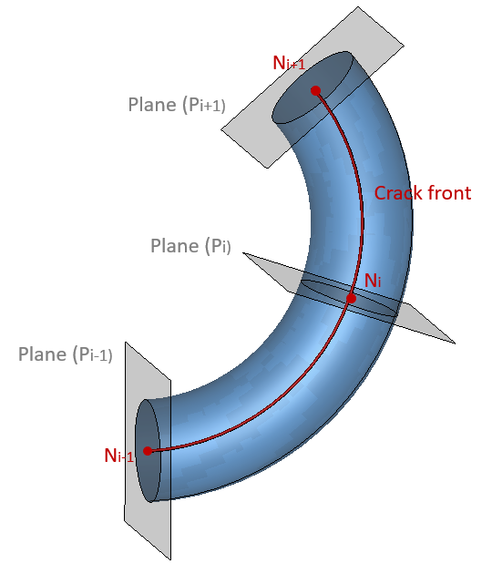
Figure 11: The local plane defined on each node of crack front in 3D.

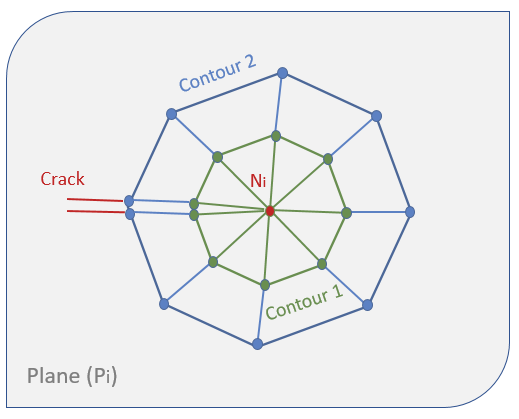
Figure 12: Definition of contour on the local plane (Pi) through the node (Ni) on crack front.

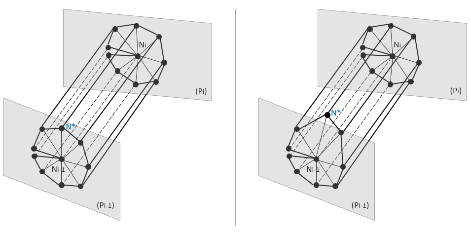
Figure 13: The defined contour on each plane in discretized problem: (left) N* node is in plane and (right) N* node is out of plane.

Identifying node and element sets within the Integral domain#

To determine the elements that compose each contour domain, POST_JMOD needs only to know the set of nodes along the crack front and the number of contours evaluated.

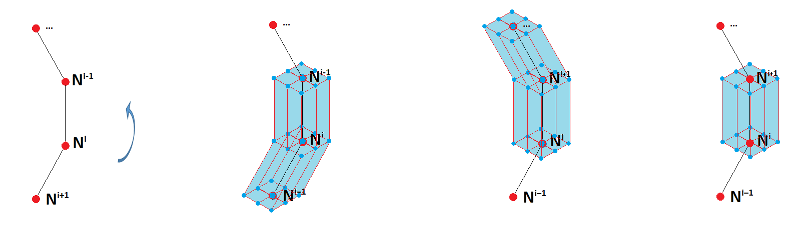
Figure 14- Domain extraction step 1. All elements with at least one node connected to the crack front are extracted for each node along the crack front. The difference in element sets between neighbouring groups is then taken.

Firstly, the nodes of the crack front are interrogated sequentially ( Figure 14 ). This allows the creation of the sub sets of elements that have at least one node contained within each of those crack front nodes. By comparing the first element set along the crack front with its neighbouring element set, the elements contained within both sets can be extracted. These elements correspond to the elements lying on the plane emanating from each crack front nodal position.

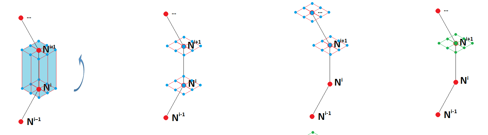
Figure 15- Domain extraction step 2. The nodes within each element set is extracted for each crack front nodal position. The neighbouring node sets are compared to obtain the intersecting nodes.

Then, the set of elements at the crack front nodal positions are interrogated sequentially ( Figure 15 ). This allows the extraction of the node sets corresponding to the element sets. The intersection between neighbouring nodal sets is used to extract the node set attached to the first contour of elements at each crack front nodal position. These nodes correspond to the nodes lying in the plane emanating from each crack front nodal position.

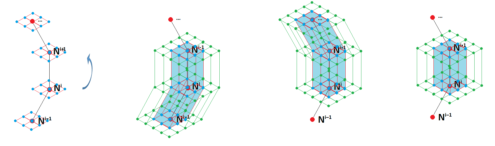
../../../../_images/10000000000006A1000001F5EB1F6948F2BCE129.png

Figure 16- Domain extraction repeat step 1 for next contour

The process is now repeated for the second contour, first allowing the extraction of elements from each crack front nodal position ( Figure 16 ), and then allowing the extraction of node sets lying in the plane emanating from each crack front nodal position ( Figure 17 ). The elements within the domain are utilised later in the POST_JMOD algorithm to perform the J computation; this is computed using with POST_ELEM command using in-built functionality to integrate over the volume (INTEGRAL). Note that only local values of J are computed along the crack front.

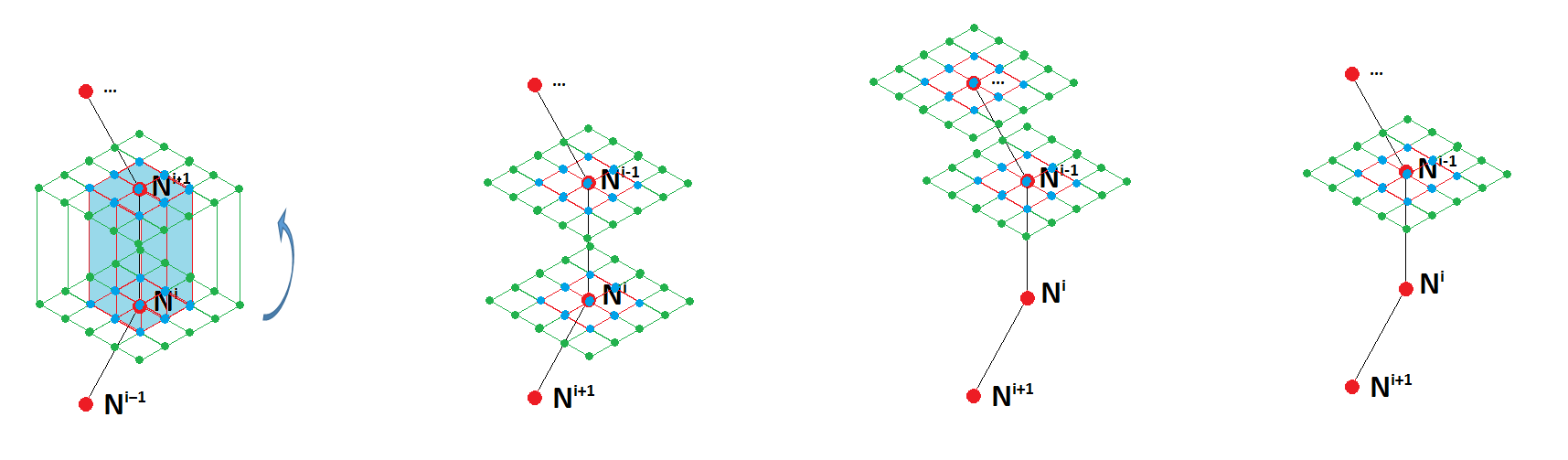
../../../../_images/10000000000006B3000001F7FFFD9B770390714E.png

Figure 17- Domain extraction repeat step 2 for next contour

The algorithm that does this makes use of in-built code_aster commands in order to define groups (or sets) of nodes and elements (DEFI_GROUP) and makes uses the specific functionality to check the difference in element sets (DIFFE) and to obtain intersections (INTERSEC). The algorithm also employs specific conditions to deal with the end most crack front nodal positions.

The domain elements and node sets are also used to assign the balues of the q -field. This allows the boundary nodes of each contour to be assigned a value of zero, and all other nodes within the contour to be assigned the virtual crack extension as a q- field.

Computation of the area increase of the cracked surface#

In a 3D analysis, J -integral takes the increase in cracked area Ac due to a virtual crack extension. This increase is due to the shift of that particular node and depends on a number of considered contours. Delorenzi [5] showed an approximate formulation for a constant strain element like 8-nodes and 20-nodes 3 D isoparametric elements but for only first contour.

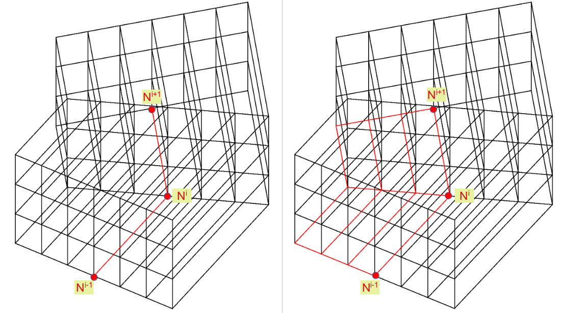
../../../../_images/100000000000045000000266992C7057F48B0247.png

Figure 18- Crack front nodes and the crack surfaces.

We present a simple case for calculating Ac at node Ni on the crack front using number of contours equal to 2 to illustrate the implementation. We consider a crack with crack front on which the node Ni and its neighbors Ni-1, Ni+1 and its surfaces are presented Figure 18 , and more clearly in Figure 19 .

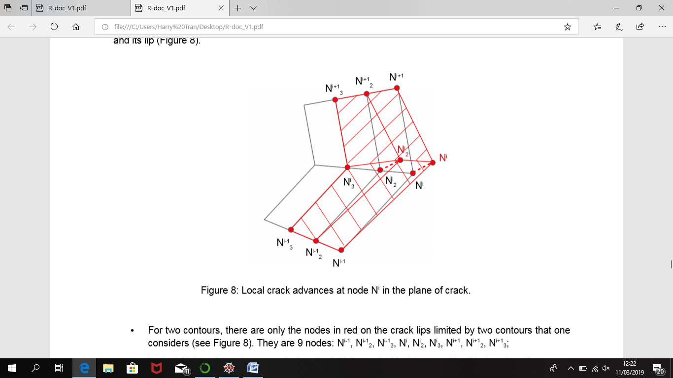
../../../../_images/1000000000000556000003005CE1CDE73305E099.png

Figure 19: Local crack advances at node Ni in the plane of crack.

For two contours, there are only the nodes in red on the crack surfaces limited by two contours that one considers (see Figure 19 ). They are 9 nodes: Ni-1, Ni-12, Ni-13, Ni, Ni2, Ni3, Ni+1, Ni+12, Ni+13;
In the initial configuration, we calculate the initial area (in black) created by these 9 nodes: Aini ;
We only move two nodes Ni and Ni2 (in black) along vector **qi* (calculated in section 2.1 ) to the new positions (in red). It is noted that only the nodes lie on the crack surface and within the integral domain (not boundary nodes) are affected by this movement;
Update the new surfaces (in red);
In this configuration, we calculate the new area (in red) created by these 9 nodes: Afin ;
The increase in cracked area Ac can be calculated:

The objective of this movement is just to calculate Ac value and the other calculations are performed on the initial mesh. To calculate Ac in POST_JMOD, we use the POST_ELEM operator with INTEGRAL option by assigning a field equal to 1 on the surface which should be calculated.

Computation of gradients of deformation terms in code_aster#

In the J -integral formulation, we need to manipulate the gradients of the displacement, the virtual crack extension (for the standard J ) and the strain (for the modified J with or without the initial strain, both proportional and non-proportional). The discretization of these fields are presented in Equations 15, 16 and 17. The components of these fields include:

displacement **u:* ( ux, uy, uz );
virtual crack extension **q:* ( qx, qy, qz );
strain **ε:* ( εxx, εyy, εzz, εxy, εxz, εyz ).

Because of the limit of Python to read the shape functions in code_aster , we use an existing principle to calculate the gradient of a field. It is noted that the strain is the results of a displacement gradient field using CALC_CHAMP operator with DEFORMATION option. It can be used when:

these fields are well determined on the nodes (TYPE_CHAM=”NOEU_XXXX_R”);
the calculation is sequentially done for each component on all components of field (3 components for u and q , and 6 components for ε ).

For example, following steps are performed to calculate the strain gradient εij,k (a non-conventional term) for the only component εxx :

\(\frac{{\partial \epsilon }_{ij}}{{\partial x}_{n}}\approx \sum_{k=1}^{\mathit{ng}}\sum_{l=1}^{3}\frac{{\partial N}_{k}}{\partial {\eta}_{l}}\frac{\partial {\eta}_{l}}{{\partial N}_{k}}{{\epsilon}_{\mathit{ijk}}|}_{\mathit{NOEU}}\) (32)

First, the strain field which was calculated at Gauss points by defaults is changed to that at the nodal points:

EPS_NOEU = CREA_CHAMP(TYPE_CHAM=”NOEU_EPSI_R”, OPERATION=”DISC”, MODELE=MODE, CHAM_GD=EPS_ELGA)

The strain field EPS_NOEU have 6 components: “EPXX”, “EPYY”, “EPZZ”, “EPXY”, “EPXZ” and “EPYZ”. We only show how to calculate the gradient of “EPXX” component as the computations for the other five components are similar.

Change the strain component “EPXX” into the displacement component “DX”:

EPS_CAL = CREA_CHAMP(OPERATION=”ASSE”, MODELE=MODE, TYPE_CHAM=”NOEU_DEPL_R”, ASSE=(_F(TOUT=”OUI”, CHAM_GD=EPS_NOEU, NOM_CMP=(“EPXX”,), NOM_CMP_RESU=(“DX”,),),),)

Create a displacement field FIELD_CAL. Its value is (EPS_CAL, 0., 0.) with the components (“DX”, “DY”, “DZ”) respectively;
Create a result from this field:

RFIELD = CREA_RESU(OPERATION=”AFFE”, NOM_CHAM=”DEPL”, TYPE_RESU=”EVOL_ELAS”, AFFE=_F(CHAM_GD=FIELD_CAL, INST=inst),)

Computing gradient with CALC_CHAMP avec DEFORMATION option of RFIELD:

GRAD_FIELD = CALC_CHAMP(reuse=RFIELD, MODELE=MODE, CHAM_MATER=MATE, RESULTAT=RFIELD, DEFORMATION=(“EPSI_ELGA”),) GRAD_FIELD = CREA_CHAMP(TYPE_CHAM=”ELGA_EPSI_R”, OPERATION=”EXTR”, RESULTAT=GRAD_FIELD, NOM_CHAM=”EPSI_ELGA”,)

This field GRAD_FIELD have six components (“EPXX”, “EPYY”, “EPZZ”, “EPXY”, “EPXZ”, “EPYZ”) and based on the formulation: εij = ½ ( ui,j+ uj,i ), we can deduce the gradient results as:

ε xx,x = GRAD_FIELD.EXTR_COMP(“EPXX”, [“MAIL”,], 1) ½ * ε xx,y = GRAD_FIELD.EXTR_COMP(“EPXY”, [“MAIL”,], 1) ½ * ε xx,z = GRAD_FIELD.EXTR_COMP(“EPXZ”, [“MAIL”,], 1)

For a completed calculation of strain gradient εij,k , we make a loop from step 1 to step 6 on all components of strain ε .

Computation of strain energy density term and its gradient#

Computation of strain energy
Without initial strain, the strain energy W can be extracted from the results of calculation STAT_NON_LINE or MECA_STATIQUE

W = CREA_CHAMP(TYPE_CHAM=”ELGA_ENER_R”,

OPERATION=”EXTR”,

RESULTAT=RESU,

NOM_CHAM=”ETOT_ELGA”,

INST=inst,)

In presence of initial strain EPS0, the mechanical strain EPSI is first calculated, then the strain energy W is computed:

EPSI_TOT = CREA_CHAMP(TYPE_CHAM=’ELGA_EPSI_R”,

OPERATION=”EXTR”,

RESULTAT=RESU,

NOM_CHAM=”EPSI_ELGA”,

INST=inst,)

EPSI = CREA_CHAMP(TYPE_CHAM=”ELGA_EPSI_R”,

OPERATION=”ASSE”,

MODELE=MODE,

ASSE=(_F(CHAM_GD=EPSI_TOT, TOUT=”OUI”,

CUMUL=”OUI”, COEF_R=1.),

_F(CHAM_GD=EPS0, TOUT=”OUI”,

CUMUL=”OUI”, COEF_R=-1.),),)

CHW = CREA_CHAMP(OPERATION=”ASSE”, TYPE_CHAM=”ELGA_NEUT_R”,

MODELE=MODE, PROL_ZERO=”OUI”,

ASSE=(_F(TOUT=”OUI”, CHAM_GD=EPSI,

NOM_CMP=(“EP**”,), NOM_CMP_RESU=(“X*”,),),

_F(TOUT=”OUI”, CHAM_GD=SIGM,

NOM_CMP=(“SI**”,), NOM_CMP_RESU=(“X*”,),),

),)

CHFMUW = FORMULE(1/2* SIGM * EPSI)

W = CREA_CHAMP(OPERATION=”EVAL”,

TYPE_CHAM=”ELGA_NEUT_R”,

CHAM_F=CHFMUW,

CHAM_PARA=(CHW,),)

Computation of gradient of strain energy

In the similar way of gradient of strain in Section 2.5 , the discretization of gradient of W is defined in Equation 33 and was performed in code_aster as:

\(\frac{{\partial \epsilon }_{ij}}{{\partial x}_{n}}\approx \sum_{k=1}^{\mathit{ng}}\sum_{l=1}^{3}\frac{{\partial N}_{k}}{\partial {\eta}_{l}}\frac{\partial {\eta}_{l}}{{\partial N}_{k}}{{\epsilon}_{\mathit{ijk}}|}_{\mathit{NOEU}}\) (33)

Change the strain energy component calculated above into the displacement component “DX”:

W_CAL = CREA_CHAMP(OPERATION=”ASSE”, MODELE=MODE,

TYPE_CHAM=”NOEU_DEPL_R”,

ASSE=(_F(TOUT=”OUI”,

CHAM_GD=__WELAS_NOEU,

NOM_CMP=(“ETOT_ELGA”,)

NOM_CMP_RESU=(“DX”,),),),)

Create a displacement field FIELD_CAL. Its value is (W_CAL, 0., 0.) with the components (“DX”, “DY”, “DZ”) respectively;
Create a result from this field: