r7.01.37 Dissipative Homogenised Reinforced Concrete (DHRC) constitutive model devoted to reinforced concrete plates#
Abstract :
This documentation presents the theoretical formulation and numerical integration of the DHRCconstitutive law, acronym for « dissipative homogenised reinforced concrete » used with modelling DKTG plates. It is one of models called « global » used to thin structures (beams, plates and shells). Nonlinear phenomena such as plasticity or damage, are directly related to the generalized strains (extension, curvature, distortion) and generalized stresses (membrane forces, bending and cutting edges). So, this constitutive law is applied with a finite element plate or shell. Compared to a multi-layered approach, CPU time and memory are saved. The advantage over multi-layer shells is even more important when the constituents of the plate behaves in a quasi-brittle manner (concrete, for example), as the global model avoids localization issues.
The DHRCconstitutive law idealises both damage and irreversible deformation under combined membrane stress resultant and bending of reinforced concrete plates using « homogenised » parameters. This constitutive law represents an evolution of the GLRC_DMconstitutive model which idealises only damage in membrane and bending situations. Unlike GLRC_DM, the DHRCconstitutive model has a complete theoretical justification by using the theory of periodic homogenization: it idealises the effects of steel-concrete slip in addition to the degradation of stiffness from the concrete diffuse cracking, the bending-membrane coupling in a consistent way and accounts for the orthotropy and possible asymmetries coming from steel reinforcement grids. The DHRCmacroscopic constitutive law is not softening: this avoids solving problems throughout the structural analysis.
The parameter setting of this constitutive law results of the particular characteristics of concrete and steel materials used, and the geometrical characteristics of the section, the thickness ratio of steel rebar, positions and directions, which are input data of a identification procedure from the responses of representative elementary volumes of the section of the reinforced concrete plate. The total user parameter number is \(21\) : \(11\) geometrical parameters and \(10\) material parameters.
Formulation of the constitutive law#
Actual problem and modelling assumptions#
We consider a concrete panel reinforced by two steel grids located on one side and the other of the middle plane of the plate. The thickness \(H\) of the plate is considered to be small compared to its overall lateral dimensions \({L}_{1}\) and \({L}_{2}\) , see figure Fig. 260, and the grids are composed with a periodic pattern of natural periodicity along \({e}_{{x}_{1}}\) and \({e}_{{x}_{2}}\) directions of the same length order as \(H\) . Moreover we consider that external loading and inertia forces spatial distributions are “smooth” with respect to the thickness \(H\) of the plate and restricted to the low frequencies range, as usual for seismic studies. Thus, it is possible to define a Reference Volume Element (RVE), denoted hereafter by \(\Omega\) , including both concrete and steel grids, whose lateral dimensions are \({l}_{1}\) and \({l}_{2}\) , see figure Fig. 260. We assume that the ratio of the lateral dimensions \({l}_{1}\) or \({l}_{2}\) over the dimensions \({L}_{1}\) or \({L}_{2}\) of the whole plate is of the same length order as the ratio of the plate thickness \(H\) over its lateral dimensions.
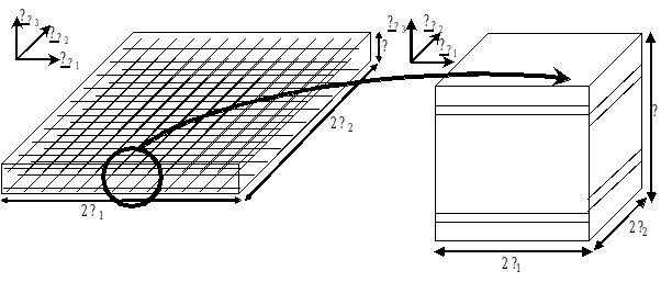
Fig. 260 RVE \(\Omega\) definition from the actual RC plate geometry#
We are interested in deriving an overall macroscopic plate constitutive relation and the previous geometrical characteristics lead us to use a multi-scale analysis or a homogenisation technique, as it was already proposed in the literature for many decades. In the case where components are assumed to be linear elastic, this multi-scale approach has been justified by using an asymptotic expansion method on three-dimensional elasticity equations. It leads to the well-known bi-dimensional linear Love-Kirchhoff’s thin plate theory if the dimensionless size of heterogeneities is of the same order that the relative slenderness of the solid, [bib16].
Both periodicity directions \({e}_{{x}_{1}}\) and \({e}_{{x}_{2}}\) ,corresponding to steel grid rebar directions, will be preferred directions for the sequel of this document. The chosen microscopic coordinate system will be the steel grid coordinate system \((O,{e}_{{x}_{1}},{e}_{{x}_{2}},{e}_{{x}_{3}})\) , where \({e}_{{x}_{3}}={e}_{{X}_{3}}\) and \(O\) is the centre of the considered RVE. The plane \({x}_{3}=0\) is the mid-plane of the RVE.
Upper and lower faces of the RVE are assumed to be free of charge, see [bib16].
Given the fact that material considerations for the actual RC plate problem are complex, several simplifications have been proposed. As reported in Suquet’s work (Suquet, 1993), the essential properties of the macroscopic homogenised model are directly defined from average energetic quantities that are computed from microscopic corresponding ones in the RVE and from some optimisation arguments associated to local thermodynamic equilibrium – especially in the standard generalised materials context (Halphen & Nguyen, 1975). Therefore, it is believed that average quantities can catch with a reasonable good agreement the overall behaviour of an actual RC plate, even if the detail of microscopic phenomena is roughly idealised. The constitutive hypothesis about materials and their bond behaviours, needed to formulate the mathematical expression of the model are listed below with their justifications
Materials behaviour in RVE \(\Omega\)#
Hyp 1 . Steel is considered linear elastic, without irreversible plastic strains, as we do not consider ultimate states of the RC plate. We denote by \({a}^{s}\) the corresponding elastic tensor.
Hyp 2.Concrete is considered elastic and damageable, according to the following constitutive model \(\text{}\sigma ={a}^{c}(d):\text{}\varepsilon\) , \(d\) being a scalar damage variable idealising distributed cracking. The associated induced anisotropy is modelled through a suitable definition of \({a}^{c}(d)\) . Concrete rigidity tensor \({a}^{c}(d)\) is defined by its initial undamaged value \({a}^{c}(0)\) , whose components are reduced by a decreasing convex damage function \(\xi (d)\) . We will give more details about the concrete constitutive model in r7.01.37-identification-approach.
Steel-concrete interface in RVE \(\Omega\)#
Hyp 3 . Concrete and steel rebar can slide one on the other beyond a given threshold.
Hyp 4 . The bond status at steel-concrete interface is either sticking or sliding. Normal separation is not allowed. We do not consider any interface elastic energy associated to the sliding motion.
Hyp 5 . The relative steel-concrete sliding, appearing after concrete damage and transmission of internal forces from concrete to steel rebar, can occur only in the two preferred directions \({e}_{{x}_{1}}\) and \({e}_{{x}_{2}}\) – along longitudinal rebar. It can differ whether considering the bar of the upper grid or of the lower grid, thus allowing to take into account its consequence on the RC plate flexural behaviour. Let’s denote by \({\Gamma}_{b}\) the generic steel-concrete interfaces along \({e}_{{x}_{1}}\) or \({e}_{{x}_{2}}\) .
Hyp 6 . Steel rebar orthogonal to the sliding direction – i.e. either perpendicular grid rebar or transversal rebar – are considered to prevent relative sliding. As a consequence, steel-concrete sliding is periodical with a period equal to the spacing between two consecutive grid bars in the considered sliding direction. This defines the lateral dimensions of the RVE \(\Omega\) .
Non-uniform damage in RVE \(\Omega\)#
Hyp 7. In order to idealise the non-uniform damage distribution of concrete along the steel rebar, concrete domain in the RVE is in fact divided into two sub-domains associated respectively to sound concrete and damaged one. Therefore, we define a whole RVE partition into two sub-domains \({\Omega}_{\mathrm{sd}}\) and \({\Omega}_{\mathrm{dm}}\) , respectively. The \({\Gamma}_{s}\) interface between these two sub-domains is assumed to be totally stuck.
Actually, concrete of the plate is not damaged in a uniform way in its volume. In order to idealise this phenomenon, one should introduce a non-uniformly distributed damage variable d in the whole RVE. Nevertheless, according to the Suquet’s work (Suquet, 1987), this non-uniformity of the microscopic internal variable field leads to the necessity to consider an infinite number of macroscopic internal variables at each macroscopic material point. This issue prevents the practical use of the macroscopic standard generalised model that would result from the chosen microscopic ones. However, still according to (Suquet, 1987), it is possible to reduce this number of internal variables to a finite one if it can be demonstrated that these internal variables are uniform or piecewise uniform or more generally described by a vector space of finite dimension. The standard generalised character of the macroscopic model is obtained from the microscopic scale behaviours thanks to the usual properties of Caratheodory’s functions of Convex Analysis. Thus, if such a chosen set of internal variables can represent the actual material state in the RVE, with a sufficient approximation degree, it is possible to build a macroscopic standard generalised model with a finite number of macroscopic internal variables. In our study, in order to restrict the number of macroscopic internal variables, we decided to define only one microscopic internal variable d for damage, considered as piecewise uniformly distributed inside the whole RVE and two sets of materials representing two different states of damage in concrete located in sub-domains \({\Omega}_{\mathrm{sd}}\) and \({\Omega}_{\mathrm{dm}}\) . This distribution of microscopic damage allows in a simple way the representation of the “tension-stiffening” effect (Combescure et al., 2013). The values of microscopic and macroscopic internal variables \(d\) and \(D\) are then equated, for the sake of simplicity, without losing any generality, since the only matter is the actual value of the respective elastic stiffness tensors.
Hyp 8 . In order to take into account the a priori non-uniform damage in the RVE thickness, two damage variables will be set up corresponding to the piecewise damage in the upper and lower halves of the RVE.
This leads to a macroscopic damage also decomposed into two macroscopic variables \({D}^{1}\) and \({D}^{2}\) .
This strong hypothesis of microscopic damage variable stepped distribution is about to represent common experimental observations during four points bending tests on RC plates: cracks opened in tension parts of the plate appear and propagate dynamically quasi-instantaneously through about the half of thickness. This crack propagation time scale is much smaller than the one considered in seismic analysis and it is then adequate to separate damage into two variables depending on the position \({x}_{3}\) in the plate thickness. The distinction between those two damage steps is chosen to be at the exact middle plane \({\Gamma}_{m}\) of the plate, being the perfectly stuck interface between upper and lower halves of the RVE. This strong approximation is in accordance with reinforced concrete design standards and regulations where it is advised to consider only half of the concrete section, for bending design, e.g. (CEB-FIP Model Code 1990, 1993). In the sequel, microscopic and macroscopic damage variables will be respectively noted \({d}^{\zeta}\) and \({D}^{\zeta}\) depending if the considered variable is the one of the upper (\(\zeta =1\) ) or lower (\(\zeta =2\) ) half of the RVE, see figure Fig. 261 .
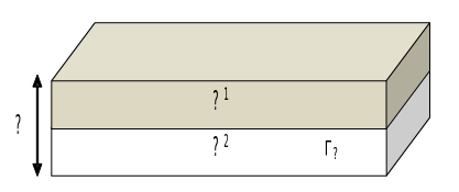
Fig. 261 Depiction of the microscopic damage variable \(d\) discretised in the RVE thickness#
Once admitted this distinction between upper and lower halves of the RVE, sub-domains \({\Omega}_{i}\) (\(i=\mathrm{sd},\mathrm{dm}\) , according to the damage status) and steel-concrete interfaces \({\Gamma}_{b}\) must be split respectively in \({\Omega}_{i}^{1}\) , \({\Omega}_{i}^{2}\) and \({\Gamma}_{b}^{1}\) , \({\Gamma}_{b}^{2}\) . Interfaces \({\Gamma}_{b}^{1}\) and \({\Gamma}_{b}^{2}\) will then be denoted by \({\Gamma}_{b}^{\zeta}\) , with \(\zeta =1,2\) .
Non-uniform steel-concrete debonding in RVE \(\Omega\)#
Let’s consider, in the RVE sketched at figure Fig. 262, that sliding can occur at steel-concrete interfaces \({\Gamma}_{b}^{\zeta}\) along the \({e}_{{x}_{1}}\) or \({e}_{{x}_{2}}\) directions.
The shapes of sliding functions \({\eta}^{\zeta}(x)\) at the interfaces \({\Gamma}_{b}^{\zeta}\) should result from the mechanical energy minimisation and then depends on the loading history in the RVE. Thus, they remain unknown before the introduction of macroscopic loading over the whole plate and cannot be determined a priori. As a consequence, the choice is made to prescribe a priori shapes for these functions in order to process conveniently to the periodic homogenisation with a limited number of variables. Moreover, as well as damage has been be chosen piecewise uniform inside the whole unit cell, it appears necessary to define sliding along each rebar from one only parameter per direction and per grid. Several possibilities can then be chosen: either the tangential displacement gap corresponding to the sliding is constant, either bond-stress induced by this sliding are. According to (Marti et al. 1998), debonding induced stress are assumed to be piecewise constant.
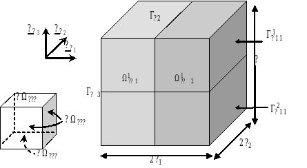
Fig. 262 Depiction of the sub-domains within the RVE thickness#
Hyp 9 .Considering the previous observation from (Marti et al 1998), a bilinear sliding function (sketched at figure Fig. 263) is chosen – corresponding to piecewise bond stresses at the interface \({\Gamma}_{b}^{\zeta}\) . This sliding function is only parameterised by its amplitude, its periodicity being fixed by the one of the RVE.
Hyp 10. Moreover, it will be considered that steel-concrete sliding vector in the \(e({x}_{\alpha})\) direction, denoted by \({\eta}_{\alpha}^{\zeta}\) , depends only on the \({x}_{\alpha}\) coordinate: it takes the same value at any point located at the steel-concrete interface \({\Gamma}_{b}^{\zeta}\) for a given \({x}_{\alpha}\) . Let’s denote by \({\stackrel{ˆ}{\eta}}_{\alpha}^{\zeta}({x}_{\alpha})\) the sliding function of unitary amplitude for the \(e({x}_{\alpha})\) direction. As a result: \({\stackrel{ˆ}{\eta}}_{\alpha}^{\zeta}({x}_{\alpha})={E}_{\alpha}^{\eta \zeta }.{\stackrel{ˆ}{\eta}}_{\alpha}^{\zeta}({x}_{\alpha}).e({x}_{\alpha})\) , \({E}_{\alpha}^{\eta \zeta }\) being its amplitude. Moreover, we observe that \(\frac{1}{{l}_{\alpha}}{\int}_{-{l}_{\alpha}}^{{l}_{\alpha}}{\stackrel{ˆ}{\eta}}_{\alpha}^{\zeta}{\mathrm{dx}}_{\alpha}=1\) .
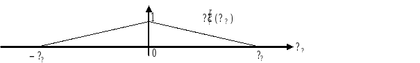
Fig. 263 Periodic sliding shape function distribution \({\stackrel{ˆ}{\eta}}_{\alpha}\) along the \(e({x}_{\alpha})\) direction with unitary amplitude in the RVE#
Overall strains measures and macroscopic state variables on RVE \(\Omega\)#
Now, according to the previous selection of phenomena to be idealised, we have to define a set of independent state variables, able to describe the mechanical state evolutions of the RC plate structural element at the macro-scale. First of all, the local microscopic displacement field \(u\) in the RVE \(\Omega =\text{}\cup {\Omega}_{i}^{\zeta}\) (\(i=\mathrm{sd},\mathrm{dm}\) in concrete, and \(i=s\) in steel rebar) is split into a regular part \({u}^{r}\) and a discontinuous one \({u}^{d}\) , associated with the debonding relative displacement defined by the \({\eta}_{\alpha}^{\zeta}\) functions (Hyp 10) at the steel–concrete interfaces \({\Gamma}_{b}^{\zeta}\) .
The overall strains measures defined as the result of the homogenisation of thin plate are the following mean surface strain tensors of second order, according to Kirchhoff-Love’s kinematics (Caillerie & Nedelec, 1984): macroscopic membrane strain tensor \(E\) , whose components are denoted by \({E}_{\mathrm{\alpha \beta }}\) , and macroscopic bending strain tensor \(K\) (curvature at first order), whose components are denoted by \({K}_{\mathrm{\alpha \beta }}\) . As we denote by \(\varepsilon (u)\) the microscopic strain tensor associated to local displacement field \(u\) in the RVE \(\Omega =\text{}\cup {\Omega}_{i}^{\zeta}\) , the components of \(E\) and \(K\) tensors are defined by the following average linear operators from the regular part \({u}^{r}\) of the displacement field:
In the sequel, the following notation \(\text{<}\cdot {\text{>}}_{\Omega}=\frac{1}{\mid \Omega \mid }{\int}_{\text{}\cup {\Omega}_{i}^{\zeta}}\cdot ~dV\) stands for the average value of the considered field in the RVE. We can easily observe that the expressions in (4895) encompass the usual definition for homogeneous plate kinematics.
We must now deal with the non-regular part \({u}^{d}\) of the displacement field in the RVE. In the sequel \(〚.〛\) stands for the jump operator on the steel-concrete interface. So, we define the macroscopic sliding strain tensor \({E}^{\mathrm{\eta \zeta }}\) as the average of sliding on each steel-concrete interface \({\Gamma}_{b}^{\zeta}\) . First, we observe that the contribution of discontinuous displacement \({u}^{d}\) to the macroscopic strain tensors vanishes, due to Hyp 4 and Hyp 10 (Andrieux et al., 1986):
where \(\mathbf{n}\) is the outward normal at the steel-concrete interface \({\Gamma}_{b}^{\zeta}\) and \(\otimes ^{s}\) stands for the symmetrised dyadic tensor product. According to Hyp 4, the displacement discontinuity \(〚{u}^{d}〛={\eta}^{\zeta}(x)\) at the interface \({\Gamma}_{b}^{\zeta}\) does not include any opening or separation in the \(n\) direction, but only tangential sliding \({\eta}_{\alpha}^{\zeta}\) . Extending the proposed definition by (Combescure et al., 2013), the components of \({E}^{\mathrm{\eta \zeta }}\) are:
Indeed, the only non-zero components of tensor \({E}^{\mathrm{\eta \zeta }}\) are \({E}_{\mathrm{\alpha \alpha }}^{\mathrm{\eta \zeta }}\) . Vector \({E}^{\mathrm{\eta \zeta }}\) will then more conveniently be considered in the following as a first-order tensor of the plate mean surface, whose components are denoted by \({E}_{\alpha}^{\mathrm{\eta \zeta }}\) .
The macroscopic primal state variables associated to the DHRC proposed model are then: membrane strains \(E\) and bending strains \(K\) tensors, damage variables \({D}^{\zeta}\) on upper and lower halves of the homogenised plate, sliding strain \({E}^{\mathrm{\eta \zeta }}\) vectors on upper and lower grids. These variables will be used to define state functions, as the macroscopic free energy density \(W(E,K,{D}^{\zeta},{E}^{\eta \zeta })\) .
Weak form of the auxiliary problems and homogenised model#
Local auxiliary problems#
In order to determine the macroscopic constitutive relation, we have to establish the relation between microscopic fields and macroscopic ones, for various fixed values of internal state variables. This relation concerns displacements fields, strain work density and dissipation potentials.
At the RVE level, as a consequence of equalities (4895) and (4897) let’s introduce two microscopic auxiliary displacement fields:
“elastic” displacement fields in membrane \(\chi\) and bending \(\xi\) corresponding to a given non-zero macroscopic strain tensor – \(E\) in membrane and \(K\) in bending – with zero sliding (\({E}^{\mathrm{\eta \zeta }}=0\) );
“sliding” displacement fields \({\chi }^{{\eta}_{\alpha}^{\zeta}}\) , corresponding to vanishing macroscopic strains (\(E=0\) , \(K=0\) ) corresponding to a given sliding function \({\eta}_{\alpha}^{\zeta}({x}_{\alpha})\) or equivalently a given \({E}_{\alpha}^{\mathrm{\eta \zeta }}\) , as done in (Andrieux et al 1986; Pensée & Kondo 2001).
Hence the microscopic displacement field \(u\) , solution of the local boundary value problem in the RVE, can be decomposed as follows (omitting intentionally the solid motion to shorten the expression):
We define the following functional spaces for displacement fields in \(\Omega\) (Caillerie & Nedelec, 1984):
and:
Remark 1:
We can easily prove that \({\langle \varepsilon (v)\rangle }_{\Omega}={\langle {x}_{3}\varepsilon (v)\rangle }_{\Omega}=0\) for any \(v\) in \({U}_{\mathrm{ad}}^{0}\) due to the periodicity and, using equations (2-3), that \({\langle \varepsilon (v)\rangle }_{\Omega}={\langle {x}_{3}\varepsilon (v)\rangle }_{\Omega}=0\) for any \(v\) in \({U}_{\mathrm{ad}}^{\mathrm{\alpha \rho }}\) .
Strain work density at the macroscopic scale is obtained by the exploitation of extended Hill-Mandel’s principle (Sanchez-Palencia, 1987; Suquet, 1987), extended to thin plate case by (Caillerie & Nedelec, 1984). Generalised stress resultants, dual of the primal overall strain variables \(E\) , \(K\) , and \({E}^{\mathrm{\eta \zeta }}\) are respectively denoted by: \(N\) , \(M\) and debonding stress vector \({\Sigma}^{\eta \zeta }\) . Macroscopic strain work balance reads:
Introducing Hyp 1 and Hyp 2 assumptions about the material behaviours within the RVE, the overall strain variables definition (cf. r7.01.37-overall-strains-measures), and the microscopic displacement field decomposition (4900) in the strain work balance (4903), microscopic periodic auxiliary displacement fields satisfy the following ten linear elastic auxiliary problems, defined in the RVE, the damage state \({d}^{\zeta}\) being fixed (subscript \(k=c\) or \(s\) , for concrete or steel):
i.e. three problems in membrane, three ones in bending and the last four associated to sliding.
Thus, any microscopic displacement field \(u\) can be expressed with the help of the previous ten auxiliary fields, by linear superposition (4900). Thanks to these results, macroscopic strain work density can be written in terms of macroscopic state variables.
Macroscopic homogenised model#
In the following we shall adopt the notation: \({\langle \langle \cdot \rangle \rangle }_{\Omega}=\frac{H}{\mid \Omega \mid }{\int}_{\text{}\cup {\Omega}_{i}^{\xi}}\cdot \mathrm{dV}\) for the average value per plate surface unit of the considered field in the RVE \(\Omega\) , \(H\) being the plate thickness, identical to the one of the RVE. The macroscopic homogenised model is obtained through the usual exploitation of extended Hill-Mandel’s principle applied to get the macroscopic Helmoltz’ free energy surface density \(W(E,K,{D}^{\zeta},{E}^{\eta \zeta })\) of the plate constitutive model. This equates the average \({\langle \langle {w}^{i}(\epsilon (u),{d}^{\zeta})\rangle \rangle }_{\Omega}\) of the microscopic free energy densities in the RVE, where, accordingly to assumptions Hyp 1 and Hyp 2:
with \(k=c\) or \(s\) , for concrete or steel. In the following, we will omit this superscript to ease writing.
After solving of the ten elastic linear independent auxiliary problems (4904) (in practice by numerical analysis), the macroscopic free energy density can be expressed as follows, using expressions (4900), depending on the macroscopic strain tensors \(E\) , \(K\) , and on the macroscopic damage and sliding internal variables \(D\) and \({E}^{\mathrm{\eta \zeta }}\) , respectively, given with fixed values:
Therefore, we can identify three homogenised behaviour tensors \(A\) , \(B\) , \(C\) of respectively fourth, third and second order, defined in the tangent plane of the plate as:
in which pure membrane (\(\mathrm{mm}\) ), pure bending (\(\mathrm{ff}\) ) and membrane-bending (\(\mathrm{mf}\) ) terms are particularised:
Remark2:
First terms in the expressions (4288) and (4290) correspond to the mixture rule; the second terms can be equivalently expressed using the variational formulations (4904) as reported here. Moreover, resulting from the symmetries of elastic tensor a, we note directly from these expressions the following symmetries: \({A}_{\mathrm{\alpha \beta \gamma \delta }}^{\mathrm{mm}}={A}_{\mathrm{\gamma \delta \alpha \beta }}^{\mathrm{mm}}\) , \({A}_{\mathrm{\alpha \beta \gamma \delta }}^{\mathrm{ff}}={A}_{\mathrm{\gamma \delta \alpha \beta }}^{\mathrm{ff}}\) , \({A}_{\mathrm{\alpha \beta \gamma \delta }}^{\mathrm{mf}}={A}_{\mathrm{\gamma \delta \alpha \beta }}^{\mathrm{mf}}\) , \({B}_{\mathrm{\alpha \beta \gamma }}^{\mathrm{m\zeta }}={B}_{\mathrm{\beta \alpha \gamma }}^{\mathrm{m\zeta }}\) , \({B}_{\mathrm{\alpha \beta \gamma }}^{\mathrm{f\zeta }}={B}_{\mathrm{\beta \alpha \gamma }}^{\mathrm{f\zeta }}\) , \({C}_{\mathrm{\alpha \gamma }}^{\mathrm{\rho \rho }}={C}_{\mathrm{\gamma \alpha }}^{\mathrm{\rho \rho }}\) .
As expected, this free energy density \(W\) has major symmetry for membrane-bending terms. Moreover, it includes a coupling term \(B\) between generalised strain tensors and bond sliding vectors that depends on damage and hence strongly couples both types of internal state variables (damage and sliding).
Remark 3:
The free energy density (4287) can also be written equivalently as:
where: \({Q}^{\zeta}(D)={A}^{(-1)}(D):{B}^{\zeta}(D)\) . and \({P}^{\mathrm{\rho \zeta }}(D)={C}^{\mathrm{\rho \zeta }}(D)-{({B}^{\rho})}^{T}(D):{A}^{(-1)}(D):{B}^{\zeta}(D)\)
This expression emphasises the existence in the presented free energy density of a coupling term between damage and sliding through an inelastic strain \({E}^{\mathrm{IR}}(D)=\left( \begin{array}{}{Q}^{\mathrm{m\zeta }}(D)\\ {Q}^{\mathrm{f\zeta }}(D)\end{array}\right).{E}^{\mathrm{\eta \zeta }}\) depending on damage variables. As observed in (Combescure et al., 2013), this constitutes a feature that is justified by the homogenisation procedure from microscopic constitutive behaviour. It makes this model differ from usual constitutive models coupling damage and plasticity (Nedjar, 2001; Chaboche, 2003; Krätzig & Pölling, 2004; Shao et al., 2006; Richard & Ragueneau, 2013…) where it is more common to refer to an inelastic residual strain \({E}^{\mathrm{IR}}\) independent of damage. Conversely, the present feature can be found in the work of (Andrieux et al., 1986), for the same reason, through homogenisation process.
Remark 4:
Expression (4286) of the free energy density is a natural generalisation, dedicated to plate structures, of the one-dimensional formulation proposed by (Combescure, Dumontet, & Voldoire, 2013) and remembered here:
\(\Phi (E,D,{E}^{\eta})=(A(D).{E}^{2})/2-B(D).{\mathrm{E.E}}^{\eta}+(C(D).{{E}^{\eta}}^{2})/2\) .
Remark 5:
It is possible to prove that coupling tensor \(B\) is equal to zero as long as the microscopic stiffness tensor \(a(d)\) is identical in both sub-domains \({\Omega}_{\mathrm{sd}}\) and \({\Omega}_{\mathrm{dm}}\) , see section 7.3, meaning that it deals with the case where damage is uniformly distributed at microscopic scale, in the whole RVE. This was observed in (Combescure et al., 2013) too and confirms experimental fact concerning the tension-stiffening effect or stress transfer from rebar to concrete induced by the non-uniformity of damage distribution at local scale .
According to the theoretical framework of the Thermodynamic of Irreversible Process, the free energy density (4286) can be differentiated to obtain the following thermodynamic forces and state laws:
Stress resultants on the homogenised plate (membrane and bending):
Using Voigt’s notation for matrices, this reads:
Macroscopic energy restitution rates \({G}^{\rho}\) :
Macroscopic debonding stress vector \({\Sigma}^{\eta \zeta }\) :
Using Voigt’s notation for matrices, with \((x,y)\) denoting the local rebar axes and \((1,2)\) the upper and lower steel grids, this reads:
Now, we have to define the dissipative behaviour at the macroscopic scale from local behaviours within the RVE. Standard Generalised material theoretical framework (Halphen & Nguyen, 1975) is adopted to express pseudo-potentials of dissipation at the microscopic scale, in order to take advantage of properties from Convex Analysis. Following the work by (Suquet, 1987), we get the macroscopic pseudo-potentials of dissipation depending on the rates of variables \({D}^{\zeta}\) , \({E}^{\mathrm{\eta \zeta }}\) , by the same average principle as done for the free energy density.
Hyp.11 : For the sake of simplicity, dissipative phenomena considered at the microscopic scale, within the RVE, are defined with the following threshold functions for concrete damage and steel-concrete debonding (assuming constant threshold parameters \({k}_{0}\) and \({\sigma}_{\mathrm{crit}}\) , without hardening…), and the associated normality rules. We assume that threshold positive parameter \({\sigma}_{\mathrm{crit}}\) is the same for all steel rebar in the RVE, whatever the bar diameter (it could be easily enhanced). Then, threshold functions read:
where \({g}^{\zeta}=-\frac{{\partial w}^{c}}{\partial {d}^{c}}\) is the microscopic energy restitution rate for damaged concrete in domain \({\Omega}_{\mathrm{sd}}^{\zeta}\) and \({\Omega}_{\mathrm{dm}}^{\zeta}\) and \({\sigma}_{\mathrm{\alpha n}}^{\zeta}\) are the tangential components of microscopic stress vector \(\sigma .n\) at the \({\Gamma}_{b}^{\zeta}\) interface. These threshold functions define convex reversibility domains.
Remark 6:
The microscopic damage threshold function results from the chosen damage model quoted in Hyp 2 and not explicitly defined until now. The sliding threshold function results from Hyp 3 and Hyp 4 .
By means of the Legendre-Fenchel’s transform applied on the indicatrix functions of previously defined reversibility domains, we get the following pseudo-potentials of dissipation:
These pseudo-potentials are convex, positively homogeneous of degree one, ensuring the positivity of dissipation for any admissible rates of damage internal variables \({\dot{d}}^{\zeta}\) and sliding ones \({\dot{\eta}}_{\alpha}^{\zeta}({x}_{\alpha})\) (Hyp 10) at steel-concrete interfaces \({\Gamma}_{b}^{\zeta}\) , according to the Clausius-Duhem’s inequality;
Associated flow rules corresponding to the sub-gradients of threshold functions (4301) give the rates of damage variables in \({\Omega}_{\mathrm{dm}}^{\zeta}\) and sliding variables at \({\Gamma}_{b}^{\zeta}\) :
where \({\dot{\lambda}}_{{d}^{\zeta}}\) and \({\dot{\lambda}}_{{\eta}^{\zeta}}^{\alpha}\) are all positive scalars determined through the consistency condition: \({\dot{f}}_{{d}^{\zeta}}=0\) and \({\dot{f}}_{{\eta}^{\zeta}}^{\alpha}=0\) . Therefore:
Now, we can express dissipation pseudo-potential functions associated to macroscopic criteria (yield surfaces), being non-negative in actual evolutions and assumed to be positively homogeneous of degree one in terms of the internal variables rates, and the internal variables flow rules. According to the work of (Suquet, 1987) and inspired from (Stolz, 2010), the macroscopic mechanical intrinsic dissipation can be defined as follows:
Where \(w(\epsilon ,{d}^{\rho})\) is the free energy density of each material composing the RVE; let us notice that \({w}_{,\epsilon }:{\epsilon}_{,{\eta}^{\zeta}}\) designates the stress vector at the concrete-steel interface.
Remark 7:
Once again, this is a generalisation, dedicated to plate structure model, of the one-dimensional formulation proposed by (Combescure et al., 2013).
According to (Suquet, 1987), we define the macroscopic pseudo-potentials of dissipation associated to damage and bond-sliding by the average on the RVE of their microscopic corresponding expressions (4302), and accounting for Hyp 10:
These convex, positively homogeneous of degree one, macroscopic pseudo-potentials of dissipation are the Legendre-Fenchel’s conjugate functions of indicatrix functions of reversibility domains at the macroscopic scale. Macroscopic threshold functions can then be identified from the macroscopic mechanical intrinsic dissipation as:
where the macroscopic strengths are given by:
Therefore, we get two damage macroscopic strengths (upper and lower halves of the RVE) and four bond sliding ones (one for each steel rebar). Finally, macroscopic flow rules take the form of normality rules, since the standard generalised properties at micro-scale are simply transferred to the macro-scale:
where \({\dot{\lambda}}_{({d}^{\rho})}\) and \({\dot{\lambda}}_{{\eta}^{\zeta}}^{\alpha}\) are all positive scalars determined through the consistency conditions: \({\dot{f}}_{({d}^{\rho})}=0\) and \({\dot{f}}_{({\eta}^{\zeta})}^{\alpha}=0\) .
Remark 8:
Macroscopic threshold functions and flow rules are similar to their microscopic homonyms modulo a scaling factor. Indeed, dissipative phenomena at the microscopic scale are naturally similar to the one located at the macroscopic scale since the homogenisation process cannot create news dissipative sources (Suquet, 1987). According to the work of (Suquet, 1987), the considered microscopic internal damage and sliding variables being uniform or piecewise constant in the whole unit cell, one can affirm, thanks to the arguments of convex analysis, that the standard generalised properties of materials, at the microscopic scale, are transferred to the macroscopic homogenised model. Hence, the formerly presented model with its free energy density and pseudo-potentials of dissipation can be classified as a Standard Generalised model .
Remark 9:
Since microscopic and macroscopic threshold functions are similar, it is possible to choose enriched threshold functions for microscopic damage and sliding. This new choice will then immediately be translated at the macroscopic scale. However, the choice of very simple threshold functions, see Hyp 11, with one only threshold parameter restricts the number of parameters to identify. Therefore, it is expected that these simple threshold functions will be sufficient for practical applications .
Remark 10:
According to Remark 5, as tensor \(B\) vanishes if there is no damage, then \({\Sigma}^{\mathrm{\eta \zeta }}\) vanishes too and the macroscopic bond sliding threshold cannot be reached before the macroscopic damage one .
Finite Element implementation#
The non-linear DHRC constitutive model formulated for plate structural element has been implemented for a DKT-CST plate finite element family (Batoz, 1982), see [R3.07.03], allowing a rather efficient and versatile modelling of complex building geometries. We remark that the curvature tensor \(K\) has opposite components in the notations used by plates elements in Code_Aster , see [R3.07.03]: the sub-matrices \({A}^{\mathrm{mf}}\) and \({B}^{f\zeta }\) have to be multiplied by \(-1\) .
The numerical integration of DHRC constitutive model lies on direct implicit time discretisation method (Nguyen, 1977), (Simo & Taylor, 1985), which is included in the Newton’ method with an elastic predictor step followed by a “plastic” corrector step, at the global balance equations stage.
At the beginning of each time step, trial generalised stresses are calculated by assuming a fully elastic response rate, with an elastic tensor evaluated for the previous damaged state. In what follows, the superscript \({\left\lbrace .\right\rbrace }^{+}\) associated to the unknown variables of the problem refers to the converged state at the end of the local integration, whereas the superscript \({\left\lbrace .\right\rbrace }^{-}\) refers to the previous converged state. It is useful to differentiate activated and non activated macroscopic mechanisms among the six possible ones – two evolving damage \({D}^{\rho}\) variables, four evolving debonding \({E}^{\mathrm{\eta \rho }}\) components – to avoid unnecessary computation. Therefore, at each Gauss point, we get back for initialising:
Then, the new internal variables are computed via a local implicit resolution of non-linear equations (flow rules) based on Newton’s method, at the \({k}^{\mathrm{th}}\) iteration:
The Jacobian matrix \(\mathbf{J}\) of all activated macroscopic threshold functions (3844) is computed by means of the closed-form expression established hereafter if all six thresholds are activated:
We recall, see (4286), that:
This matrix is diagonal, by construction of the tensors \(\mathbf{A}(D)\) , \(\mathbf{B}(D)\) , \(\mathbf{C}(D)\) .
The estimated new state is so corrected to satisfy the discretised forms of the thresholds of damage and debonding, until a prescribed tolerance is reached on each threshold. The overview of the implicit integration algorithm is drawn at figure Fig. 264. in a first step, the activated thresholds are determined. Then the rates of the corresponding internal variables are solved by the Newton’s method. The all six thresholds are verified, and if some other ones are reached, the non-linear system is updated. At the end, all the local variables are updated.
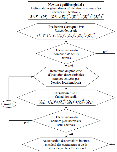
Fig. 264 Chart of the constitutive law implicit integration#
Once the calculation of the new internal variables is done, we perform the new stress resultants, see (4295) and (4296); finally one calculates the tangent stiffness operator from the first variations of tensors \(\mathbf{E}\) and \(\mathbf{K}\) and corresponding first variations of \(D\) and \({E}^{\eta \zeta }\) :
The last vectors are obtained from the inverse of the Jacobian matrix \(\mathbf{J}\) of all macroscopic threshold functions, taking advantage of consistency equations \({\dot{f}}_{({d}^{\rho})}=0\) and \({\dot{f}}_{({\eta}^{\zeta})}^{\alpha}=0\) , see equations (3846) and (4583), where superscript \(\tau\) means \(m\) or \(f\) according the case:
Parameter identification procedure#
We present in this section the general approach carried out in order to identify DHRC parameters. The needed microscopic scale data: geometry and material characteristics, and the main steps of the proposed automated procedure are detailed.
Identification approach#
The main difficulty to be overcome hereafter is to ensure that with a limited number of auxiliary problems solutions, we will be able to identify DHRC parameters that:
cover the space of macroscopic states (\(\mathbf{E}\) , \(\mathbf{K}\) , \({D}^{\zeta}\) , \({E}^{\eta \zeta }\) ),
have a generic dependency on macroscopic damage variable \({D}^{\zeta}\) , from the sound state, distinguishing tensile and compressive regimes,
ensure continuity of stress resultants (\(\mathbf{N}\) , \(\mathbf{M}\) , \({\Sigma}^{\eta \zeta }\) ) at each regime change,
ensure the convexity of the macroscopic free energy density.
We decided to perform some “snapshots” of microscopic states for a limited number of selected macroscopic ones, and to entrust the task of determining the parameters dependency to \({D}^{\zeta}\) to a least squares method and an appropriate selected function of \({D}^{\zeta}\) . We recall from (Combescure et al., 2013), that in one dimension, if the microscopic damage function, controlling the elastic stiffness degradation \({a}^{c}(d)\) , is expressed as \(\xi (d)=(\alpha +\mathrm{\gamma d})/(\alpha +d)\) (which is decreasing convex for \(\gamma \le 1\) ) then the macroscopic one-dimensional elastic tensor \(A\) follows the same dependency and is equal to \(\mathbf{A}={\mathbf{A}}^{0}({\alpha}_{A}+{\gamma}_{A}D)/({\alpha}_{A}+D)\) , with \({\gamma}_{A}\le 1\) , similarly for the other tensors \(\mathbf{B}\) and \(\mathbf{C}\) . This ensures the convexity of the resultant Helmholtz free energy function, provided that γ is not “excessively” negative.
As shown in the previous section, from the solutions of a set of auxiliary elastic problems, we have to identify the components of three tensors \(\mathbf{A}\) , \(\mathbf{B}\) and \(\mathbf{C}\) with their macroscopic damage variable \({D}^{\zeta}\) dependency. Two macroscopic threshold values for damage and sliding need also to be determined.
Hyp.12 . According to the results obtained for the macroscopic one-dimensional case (Combescure et al., 2013), we assume the generic following dependency on \({D}^{\zeta}\) variable of the macroscopic tensors components (the particular expression for tensor \(\mathbf{B}\) resulting from Remark 6):
Of course this compromise will have to be assessed by comparison of DHRC model results with available experimental data on actual RC structures and usual loading paths.
Microscopic material parameters in RVE \(\Omega\)#
According to assumptions Hyp 1, steel is considered as linear elastic (defined by its Young’s modulus \({E}_{s}\) and Poisson’s ratio \({\nu}_{s}\) ). Hyp 2 assumes that concrete is elastic and damageable. The latter is defined by the following constitutive model \(\sigma ={a}^{c}(d):\varepsilon\) , \(d\) being the microscopic scalar damage variable. In particular, we have to define damage dependency of elastic constants, how to deal with tensile and compressive regimes, the relationship with usual concrete behaviour parameters, induced anisotropy and the distribution of damaged sub-domains into the RVE according to macroscopic states
Hyp. 13. Microscopic concrete elasticity tensor \({a}^{c}(d)\) is defined by its initial sound isotropic elastic tensor \({a}^{c}(0)\) , characterised by Young’s modulus \({E}_{c}\) and Poisson’s ratio \({\nu}_{c}\) . For \(d>0\) , the elasticity tensor components are reduced by a multiplicative decreasing convex damage function \(\xi (d)\) . We propose the generic mathematical expression \(\xi (d)=(\alpha +\gamma d)/(\alpha +d)\) , with \(\gamma <1\) – ensuring a stiffness degradation for increasing damage \(d\) – which produces a bilinear strain-stress response for uniaxial monotonic loading paths, see section §4.1 of (Combescure et al., 2013).
Hyp. 14. In order to distinguish between tensile and compressive states in concrete sub-domains we introduce a dissymmetry in \(\xi (d)\) . To this end, the microscopic damage function is modified through the use of a Heaviside’s function \(H(x)\) and then takes the following form:
This means that damage function \(\xi\) includes four parameters:
In practice, we take \({\alpha}_{+}=1\) without getting out any generality, as the only consequence is to normalise the damage variable \(d\) . In addition, we will take the following set of five values of \(d\) : \(\lbrace 0.,0.5,2.,10.,20.\rbrace\) , considered to cover a sufficient range of damage for an accurate identification. This choice seems to be the better compromise between relative error and computing burden.
Concrete free energy density being \(w(\epsilon ,d)=\frac{1}{2}\epsilon :{\mathbf{a}}^{c}(d):\epsilon\) , we define energy release rate by \(g(\epsilon ,d)=-{w}_{,d}(\epsilon ,d)\) , and convex reversibility domain by the damage criterion with the constant threshold value \({k}_{0}\) , see Hyp 11 and expression (4301):
According to uniaxial stress-strain curves of concrete (CEB-FIP Model Code 1990, 1993), we use the usual following parameters: concrete tensile \({f}_{t}\) and compression \({f}_{c}\) strength values (the former being associated to a fracture energy \({G}_{f}\) , the later to a compression strain \({\epsilon}_{\mathrm{cm}}\) ) and we assume a threshold value \({f}_{\mathrm{dc}}\) of initial damage in compression. So, assuming a multilinear regression of the experimental stress-strain curve through this concrete constitutive model, we can associate the values of \({\alpha}_{-}\) , \({\gamma}_{-}\) , \({\gamma}_{+}\) and \({k}_{0}\) with usual engineering parameters \({f}_{t}\) , \({G}_{f}\) , \({f}_{c}\) , \({\epsilon}_{\mathrm{cm}}\) , \({f}_{\mathrm{dc}}\) .
Let us consider a pure tensile uniaxial membrane stress loading case \({N}_{11}^{t}\) , in the \({x}_{1}\) direction, on a sound RVE, i.e. with zero-valued internal variables: indeed the problem remains linear. Thus, referring to equations (4298) and (3845), we may express the macroscopic energy restitution rates, which is quadratic in \({N}_{11}^{t}\) :
In parallel, we calculate the microscopic energy restitution rate (3856), using (4900) to express the local strain tensor \(\epsilon\) using the generalised strain measures \(E\) , \(K\) obtained by inverting (4295) and (4296) to express them from \({N}_{11}^{t}\) :
Moreover, we calculate the stress tensor \(\sigma ={\mathbf{a}}^{c}(0):\epsilon\) field at any point within the RVE concrete domain \({\Omega}_{c}^{\zeta}\) , and we determine the maximum value \({\stackrel{ˆ}{\sigma}}_{t}^{\max}.\mid {N}_{11}^{t}\mid\) of the eigen-values of this tensor, according to a Rankine criterion. Equating with the given \({f}_{t}\) parameter, we get the critical value \({\tilde{N}}_{11}^{t}\) in tension, then the following relation, see also (3845):
Therefore, we can deduce the value of \({k}_{0}\) from \({f}_{t}\) , \({\stackrel{ˆ}{g}}_{{N}_{xx}}^{t}\) and \({\stackrel{ˆ}{\sigma}}_{t}^{\max}\) . Of course, the local quantities \({\stackrel{ˆ}{\sigma}}_{t}^{\max}\) and \({\stackrel{ˆ}{g}}_{{N}_{11}}^{t}\) are depending on \({\alpha}_{-}\) , \({\gamma}_{-}\) , \({\gamma}_{+}\) values, while the two values \({\stackrel{ˆ}{G}}_{{N}_{11}}^{t\zeta }\) (for \(\zeta =1\) and \(\zeta =2\) ) depend on the macroscopic \(A(0)\) tensor components and all the \({\alpha}^{A}\) and \({\gamma}^{A}\) parameters to express the derivative \({A}_{,{D}^{\zeta}}(0)\) .
We could easily proceed in the same manner for a pure compressive uniaxial membrane stress loading case \({N}_{11}^{c}\) . Nevertheless, we assume that it is satisfactory to follow the expression shown in section §4.2 of (Combescure, Dumontet, & Voldoire, 2013), which corresponds to a pure one-dimensional case:
(One recalls that \({\alpha}_{+}=1\) ). We propose to roughly approximate the post-elastic part of the concrete uniaxial compression curve by a linear segment ranging from the first damage threshold \({f}_{\mathrm{dc}}\) to the extremum (\({\epsilon}_{\mathrm{cm}}\) , \({f}_{c}\) ), so that \({\gamma}_{-}\) belonging to \(]0.,1.]\) . Then:
Hyp. 15. Finally, we propose to choose \({\gamma}_{+}\) so that the softening post-peak tensile path becomes sufficiently weak in order to avoid any softening of the homogenised response by the DHRC constitutive model. It is expected that provided that \({\gamma}_{+}\) remains close to zero, even negative, the homogenised free energy density will be strictly convex (this will be checked at the end of the identification process, see also section 7.2). So, we don’t make use of \({G}_{f}\) .
Hence, from (3860), we get:
Remark 11:
The series expansions at order 2 of the \(\xi (d)\) function are:
\(\begin{array}{}\xi (d)=1+\frac{\gamma -1}{\alpha}d+o({d}^{2})=\gamma +\frac{1-\gamma }{d}\alpha +o({\alpha}^{2})\\ \text{}=1+d(\gamma -1)(2-\alpha )+o({d}^{2})+o({(\alpha -1)}^{2})\end{array}\)
Therefore, in the vicinity of \(d=0\) , \(\frac{\gamma -1}{\alpha}\) controls the negative slope of \(\xi (d)\) ; so, this slope is directly inversely proportional to \(\alpha\) : it has to be kept in mind to choose the \({\alpha}_{-}\) parameter value; a priori, we can expect that \({\alpha}_{-}>1\) . For large damage values, \(\xi (d)\) tends to the asymptotic value \({\gamma}_{-}\) . Finally, around \({\alpha}_{-}=1\) value, the negative slope of \(\xi (d)\) is \({\gamma}_{-}-1\) .
Hyp. 16. Given the orthotropic geometry of the plate, we assume that damage induces orthorhombic behaviour, and define the nine orthorhombic elastic constants from the values of sound concrete Lamé’s constants \({\lambda}_{c}\) , \({\mu}_{c}\) . The principal material directions in the \(({x}_{1,}{x}_{2})\) plane are chosen according to the macroscopic membrane strain directions, respectively: at \(0°\) for the case of dilatation strains or bond sliding, at \(45°\) for the case of shear strains only.
Even if this choice could appear as arbitrary, and can be replaced by another one, it is believed that it will be satisfactory for our purposes
Hyp. 17. Variable \(x\) in equation (3854) is chosen to be macroscopic membrane strain component \({E}_{\mathrm{\alpha \beta }}\) for the diagonal terms of tensors \(\mathbf{A} ` , :math:\)mathbf{B} ` and \(\mathbf{C} ` and tensor invariant :math:\)mathrm{tr}E` for their off-diagonal terms. Therefore we are neglecting the microscopic correctors influence in the damaged elastic tensor microscopic values. Moreover, this choice keeps the needed symmetry properties of homogenised tensors \(\mathbf{A}\) , \(\mathbf{B}\) and \(\mathbf{C}\) . For bending auxiliary problems, we replace tensor \(\mathbf{E}\) by tensor \(\mathbf{K}\) . For bond sliding auxiliary problems (\({{\rm E}}_{\mathrm{\alpha \beta }}=0\) , \({{\rm K}}_{\mathrm{\alpha \beta }}=0\) , see equation (4904) tensile damage is expected in the considered concrete sub-domain of the RVE, thus parameter \({\gamma}_{+}\) is used. Consequently, we set:
For bond sliding auxiliary problems, the orthorhombic elastic constants are:
For macroscopic membrane and bending unit auxiliary problems (4904), they fulfil:
Remark 12:
Therefore, in pure shear strain case, compressive elastic constant \(\tilde{\lambda}={\lambda}_{-}\) is assigned .
Hyp. 18. Finally, we assume several distributions of concrete sub-domains within the RVE, according to the needed dissymmetry of damage distribution (Hyp 7, Hyp 8, Hyp 10). Hence we will consider the following three kinds of distributions of \({\Omega}_{i}^{\zeta}\) sub-domains (\(i=\mathrm{sd},\mathrm{dm}\) ) for sound or damaged concrete in upper or lower halves of the RVE (\(\zeta =1,2\) ), with previous isotropic elastic constants in the sound concrete \({\Omega}_{\mathrm{sd}}^{\zeta}\) sub-domains and orthotropic elastic constants (for five damage values taken in the set: \(\lbrace 0.,0.5,2.,10.,20.\rbrace\) ; we performed a sensitivity analysis whose conclusion showed that it is a good compromise) and principal material directions in the damaged \({\Omega}_{\mathrm{dm}}^{\zeta}\) sub-domains. These distributions constitute three kinds of RVE, named hereafter \({\Omega}_{X}\) , see figure Fig. 261, and \({\Omega}_{Y}\) (first principal material direction at \(0°\) in the (\({x}_{1}\) , \({x}_{2}\) ) plane), \({\Omega}_{(45°)}\) (first principal material direction at \(45°\) in the (\({x}_{1}\) , \({x}_{2}\) ) plane), see Table 4 1.
These three kinds of RVE are designed to deal with the respective directions of macroscopic loading. The \({\Omega}_{(45°)}\) RVE is used for the shear strains loading cases, where no separation in the (\({x}_{1}\) , \({x}_{2}\) ) plane is needed. So, in those cases the contribution of bond sliding vanishes, as we can deduce from the corresponding auxiliary problems. Conversely, as we need to perform cross products between corrector fields to determine the off-diagonal components of the homogenised tensors \(\mathbf{A}\) , \(\mathbf{B}\) , \(\mathbf{C}\) , we have to carry out calculations on the three kinds of RVEs for membrane and bending macroscopic strains.
RVE |
loading |
damaged half |
\({\Omega}_{i}^{\zeta}\) sub-domains |
\({\Omega}_{X}\) |
membrane, bending and bond sliding |
\({d}^{1}\ge 0\) , \({d}^{2}=0\) |
for \({x}_{3}>0\) : \({\Omega}_{\mathrm{dm}}^{1}\) for \({x}_{1}>0\) and for \({x}_{1}<0\) for \({x}_{3}<0\) : \({\Omega}_{\mathrm{sd}}^{2}\) |
\({\Omega}_{X}\) |
membrane, bending and bond sliding |
\({d}^{1}=0\) , \({d}^{2}\ge 0\) |
for \({x}_{3}>0\) : \({\Omega}_{\mathrm{sd}}^{1}\) for \({x}_{3}<0\) : \({\Omega}_{\mathrm{dm}}^{2}\) for \({x}_{1}>0\) and for \({x}_{1}<0\) |
\({\Omega}_{Y}\) |
membrane, bending and bond sliding |
\({d}^{1}\ge 0\) , \({d}^{2}=0\) |
for \({x}_{3}>0\) : \({\Omega}_{\mathrm{dm}}^{1}\) for \({x}_{2}>0\) and for \({x}_{2}<0\) for \({x}_{3}<0\) : \({\Omega}_{\mathrm{sd}}^{2}\) |
\({\Omega}_{Y}\) |
membrane, bending and bond sliding |
\({d}^{1}=0\) , \({d}^{2}\ge 0\) |
for \({x}_{3}>0\) : \({\Omega}_{\mathrm{sd}}^{1}\) for \({x}_{3}<0\) : \({\Omega}_{\mathrm{dm}}^{2}\) for \({x}_{2}>0\) and for \({x}_{2}<0\) |
\({\Omega}_{(45°)}\) |
membrane and bending |
\({d}^{1}\ge 0\) , \({d}^{2}=0\) |
for \({x}_{3}>0\) : \({\Omega}_{\mathrm{dm}}^{1}\) for any \({x}_{1}\) , \({x}_{2}\) for \({x}_{3}<0\) : \({\Omega}_{\mathrm{sd}}^{2}\) |
\({\Omega}_{(45°)}\) |
membrane and bending |
\({d}^{1}=0\) , \({d}^{2}\ge 0\) |
for \({x}_{3}>0\) : \({\Omega}_{\mathrm{sd}}^{1}\) for \({x}_{3}<0\) : \({\Omega}_{\mathrm{dm}}^{2}\) for any \({x}_{1}\) , \({x}_{2}\) |
Remark 13:
Note that the volume of damaged concrete sub-domains is \(\mathrm{¼}\) of total for both \({\Omega}_{X}\) , \({\Omega}_{Y}\) RVEs and \(\mathrm{½}\) of total for \({\Omega}_{(45°)}\) RVE .
Finally, we have to solve \(207\) auxiliary problems: nine damage (\({d}^{1}\) , \({d}^{2}\) ) values combinations (with five \({d}^{\zeta}\) values taken in the set: {0,0.5,2.,10.,20.}) times twenty-three kinds of RVE \({\Omega}_{i}^{\zeta}\) sub-domains distributions and loading conditions: nine with the \({\Omega}_{X}\) RVE according to the \({x}_{1}\) direction (five without bond sliding, four with sliding conditions), nine with the \({\Omega}_{Y}\) RVE according to the \({x}_{2}\) direction, five with the \({\Omega}_{(45°)}\) RVE with orthotropic reference frame rotated \(45°\) (without bond sliding). The following Table 4 2 sums up these cases; it is relevant also for pure macroscopic bending loading cases (\({{\rm K}}_{\mathrm{\alpha \beta }}\) instead of \({{\rm E}}_{\mathrm{\alpha \beta }}\) ), adding so fifteen times nine (\(135\) ) other elastic problems to solve.
RVE \({\Omega}_{X}\) |
RVE \({\Omega}_{Y}\) |
RVE \({\Omega}_{(45°)}\) |
macroscopic membrane strain |
macroscopic membrane strain |
macroscopic membrane strain |
\({{\rm E}}_{11}=-1\) , \({{\rm E}}_{22}=0\) , \({{\rm E}}_{12}=0\) \({{\rm E}}_{11}=1\) , \({{\rm E}}_{22}=0\) , \({{\rm E}}_{12}=0\) \({{\rm E}}_{11}=0\) , \({{\rm E}}_{22}=-1\) , \({{\rm E}}_{12}=0\) \({{\rm E}}_{11}=0\) , \({{\rm E}}_{22}=1\) , \({{\rm E}}_{12}=0\) \({{\rm E}}_{11}=0\) , \({{\rm E}}_{22}=0\) , \({{\rm E}}_{12}=0.5\) |
\({{\rm E}}_{11}=-1\) , \({{\rm E}}_{22}=0\) , \({{\rm E}}_{12}=0\) \({{\rm E}}_{11}=1\) , \({{\rm E}}_{22}=0\) , \({{\rm E}}_{12}=0\) \({{\rm E}}_{11}=0\) , \({{\rm E}}_{22}=-1\) , \({{\rm E}}_{12}=0\) \({{\rm E}}_{11}=0\) , \({{\rm E}}_{22}=1\) , \({{\rm E}}_{12}=0\) \({{\rm E}}_{11}=0\) , \({{\rm E}}_{22}=0\) , \({{\rm E}}_{12}=0.5\) |
\({{\rm E}}_{11}=-1\) , \({{\rm E}}_{22}=0\) , \({{\rm E}}_{12}=0\) \({{\rm E}}_{11}=1\) , \({{\rm E}}_{22}=0\) , \({{\rm E}}_{12}=0\) \({{\rm E}}_{11}=0\) , \({{\rm E}}_{22}=-1\) , \({{\rm E}}_{12}=0\) \({{\rm E}}_{11}=0\) , \({{\rm E}}_{22}=1\) , \({{\rm E}}_{12}=0\) \({{\rm E}}_{11}=0\) , \({{\rm E}}_{22}=0\) , \({{\rm E}}_{12}=0.5\) |
bond sliding |
bond sliding |
no bond sliding |
\({E}_{1}^{\mathrm{\eta 1}}=1\) , other zero \({E}_{2}^{\mathrm{\eta 1}}=1\) , other zero \({E}_{1}^{\mathrm{\eta 2}}=1\) , other zero \({E}_{2}^{\mathrm{\eta 2}}=1\) , other zero |
\({E}_{1}^{\mathrm{\eta 1}}=1\) , other zero \({E}_{2}^{\mathrm{\eta 1}}=1\) , other zero \({E}_{1}^{\mathrm{\eta 2}}=1\) , other zero \({E}_{2}^{\mathrm{\eta 2}}=1\) , other zero |
– |
Macroscopic material parameters to be determined#
After solving the \(342\) auxiliary problems, we have at our disposal enough information on the corrector fields \({\chi }^{\mathrm{\alpha \beta }}\) in membrane, \({\xi}^{\mathrm{\alpha \beta }}\) in bending and \({\chi }^{{\eta}_{\alpha}^{\rho}}\) for bond sliding to compute the \(A\) , \(B\) , \(C\) macroscopic tensors components, see section 3.1.2. All components are expressed in the reference frame determined by the steel bar grids.
Tensor \(\mathbf{A}\)#
Tensor \(\mathbf{A} ` is the stiffness elastic damageable tensor of the homogenised RC plate tensor, see equations :eq:`eq-3-9\), (4289), (4290) . It is a symmetric fourth order tensor of the tangent plane (see Remark 3) comprising membrane, bending and coupling terms. It is possible to store it using Voigt’s notation for tensors components in the reference frame of steel rebar grids, by means of \(3\times 3\) matrices:
From equations (4289) , we deduce that \({\mathbf{A} }^{\mathrm{mm}}\) and \({\mathbf{A} }^{\mathrm{ff}}\) matrices are symmetric, whereas in general no symmetry argument hold for \({\mathbf{A} }^{\mathrm{mf}}\) matrix. Therefore we have \(21=6+6+9\) components to be determined for tensor \(\mathbf{A}\) .
Remark 14:
If the RC plate presents mirror symmetry (symmetry around the medium plane), then both membrane-bending coupling matrices \({A}^{\mathrm{mf}}\) and \({A}^{\mathrm{fm}}\) should vanish as long as damage variables verify \({D}^{1}={D}^{2}\) .
Hyp. 19 . We define the parameters \({\alpha}^{A}\) and \({\gamma}^{A}\) characterising the dependency on macroscopic damage variable \({D}^{\zeta}\) (Hyp 12) and the tensile/compressive distinction in membrane or positive/negative curvature in bending of the tensor \(\mathbf{A}\) components (Hyp 14) by:
where the superscripts \(\mathrm{\tau \tau }\) stand for membrane or bending (\(\mathrm{mm}\) or \(\mathrm{ff}\) ), the superscript \(\varsigma\) stands for tension or compression case and tensorial subscripts \(\beta\) , \(\delta\) , \(\lambda\) , \(\mu\) stand for directions in the plate tangent plane. Discrimination between “tension” or “compression” status in membrane loading is decided either from the sign of \(x={{\rm E}}_{\mathrm{\beta \delta }}+{Q}_{\mathrm{\beta \delta }}^{m\zeta }(D).{E}^{\eta \zeta }\) if \(\mathrm{\beta \delta }=\mathrm{\lambda \mu }\) or the sign of \(x=\mathrm{tr}(E+{Q}^{m\zeta }(D).{E}^{\eta \zeta })\) , where \({Q}^{m\zeta }(D)\) is defined by (4294), and respectively with \(K\) tensor; nevertheless, we decided that the \({A}_{\mathrm{\beta \delta \lambda \mu }}^{\mathrm{mf}}\) components doesn’t include this discrimination. This choice allows avoiding any discontinuity of macroscopic stress resultant (4295) and (4296), ensuring the convexity of the strain energy density function, according to the general result shown by (Curnier, He, & Zysset, 1995). The \({A}_{\mathrm{\beta \delta \lambda \mu }}^{\mathrm{0\tau \tau }}\) and \({A}_{\mathrm{\beta \delta \lambda \mu }}^{0\mathrm{mf}}\) components correspond to the sound concrete homogenised elasticity. \({A}_{\mathrm{\beta \delta \lambda \mu }}^{0\mathrm{mf}}\) is expected to vanish in the case of mirror symmetry, as said before. That is why we decided to adopt the particular dependency on \({D}^{\zeta}\) for the \({A}_{\mathrm{\beta \delta \lambda \mu }}^{\mathrm{mf}}\) terms, see equation (3867).
Remark 15:
This special choice of \(x\) as status variable allows us to use the direct component of the strain tensor for diagonal terms and an invariant for off-diagonal ones, conserving then the symmetry of tensor \(\mathbf{A}\) *. The function distinguishing tensile or compressive status being not defined when* \(E+{Q}^{m\zeta }(D)=0\) (resp. \(K+{Q}^{f\zeta }(D)=0\) ), arbitrarily, “tension” parameters are affected to the zero macroscopic strain case.
Therefore, there is a total of \(21\times (1+2\times 4)=189\) necessary parameters \({A}_{\mathrm{\beta \delta \lambda \mu }}^{0}\) , \({\alpha}^{A}\) and \({\gamma}^{A}\) to fully determine the elastic stiffness tensor \(A\) , comprising its dissymmetric dependency on macroscopic damage variables \({D}^{1}\) and \({D}^{2}\) and on tensile or compressive status. Using the Voigt’s notation for matrices, \({A}^{0}\) reads:
In order to make easier the comparison with the GLRC_DM constitutive model [r7.01.32], we can determine equivalent membrane and bending Young’s moduli, and equivalent Poisson’s ratios:
\({E}_{\mathrm{eq}}^{\mathrm{mx}}=\frac{1}{H}\frac{{A}_{\mathrm{xxxx}}^{\mathrm{0mm}}{A}_{\mathrm{yyyy}}^{\mathrm{0mm}}-{({A}_{\mathrm{xyxy}}^{\mathrm{0mm}})}^{2}}{{A}_{\mathrm{yyyy}}^{\mathrm{0mm}}}\) ; \({E}_{\mathrm{eq}}^{\mathrm{fx}}=\frac{12}{{H}^{3}}\frac{{A}_{\mathrm{xxxx}}^{\mathrm{0ff}}{A}_{\mathrm{yyyy}}^{\mathrm{0ff}}-{({A}_{\mathrm{xyxy}}^{\mathrm{0ff}})}^{2}}{{A}_{\mathrm{yyyy}}^{\mathrm{0ff}}}\) ; \({\nu}_{m}^{x}=\frac{{A}_{\mathrm{xxyy}}^{\mathrm{0mm}}}{{A}_{\mathrm{xxxx}}^{\mathrm{0mm}}}\) ; \({\nu}_{f}^{x}=\frac{{A}_{\mathrm{xxyy}}^{\mathrm{0ff}}}{{A}_{\mathrm{xxxx}}^{\mathrm{0ff}}}\)
where \(H\) is the RC plate thickness.
Tensor \(\mathbf{B}\)#
Tensor \(\mathbf{B}\) is the coupling elastic damage-sliding tensor, see equations (4291) and (4292). It is a symmetric third order tensor of the tangent plane, comprising membrane and bending terms. It is possible to store its components using Voigt’s notation: \(\mathbf{B}=\left( \begin{array}{}{B}^{\mathrm{m\zeta }}\\ {B}^{\mathrm{f\zeta }}\end{array}\right)\) , where superscript \(\zeta\) stands for sliding in the upper (\(\zeta =1\) ) or lower (\(\zeta =2\) ) grid.
Remark 16:
While elastic membrane, and bending corrector fields have been computed for both tensile and compressive macroscopic loading, elastic corrector fields \({\chi }^{{\eta}^{\zeta}}\) are obtained for sliding displacement with zero membrane and bending macroscopic loading. Hence tensor \(\mathbf{B}\) should include a tension-compression dissymmetry. However, this could introduce a discontinuity in the expression of generalised stresses as soon as macroscopic sliding strain becomes non-zero, see equations (4295), (4296) and (4299) . Therefore, we decided to introduce no tension-compression dissymmetry in tensor \(B\) .
Hyp. 20 . Parameters \({\alpha}^{B}\) and \({\gamma}^{B}\) characterising the dependency on the macroscopic damage \({D}^{\zeta}\) (Hyp 12) without tensile/compressive distinction are defined. According to Remark 6 see also r7.01.37-proof-zero-valued , when materials are symmetric relative to the plane \({\Gamma}_{s}\) normal to the sliding bar at point \(O\) (i.e. tensor \(\mathbf{B}\) components vanish. As a consequence, there is no need to determine “elastic” properties for this tensor. Thus we state:
where the superscript \(\tau\) stands for membrane or bending (\(m\) or \(f\) ), the superscript \(\zeta\) stands for the zone where sliding takes place (upper or lower), tensorial subscripts \(\beta\) , \(\delta\) stand for membrane or bending directions in the plate tangent plane while tensorial subscript \(\lambda\) stands for sliding strain \({E}_{\lambda}^{\mathrm{\eta \zeta }}\) . There is, with a fixed sliding zone, \(6\) components for tensors \({B}^{\mathrm{m\zeta }}\) and \({B}^{\mathrm{f\zeta }}\) so \(24\) components for the whole tensor \(\mathbf{B}\) . Therefore, there is a total of \(24\times (2\times 2)=96\) necessary \({\alpha}^{B}\) and \({\gamma}^{B}\) parameters to fully determine the coupling elastic damage-sliding tensor \(\mathbf{B}\) .
Tensor \(\mathbf{C}\)#
Tensor \(\mathbf{C}\) is the sliding elastic “stiffness” tensor, computed from the four \({\chi }^{({\eta}_{\alpha}^{\rho})}\) sliding auxiliary fields, see equation (4293). It is a second order symmetric tensor of the tangent plane of the plate: \({C}_{\mathrm{\lambda \mu }}^{\mathrm{\rho \zeta }}={C}_{\mathrm{\mu \lambda }}^{\mathrm{\rho \zeta }}\) (Remark 3). It is possible to store \(C\) components using Voigt’s notation. The number of components of tensor \(C\) is then \(10\) : sliding along \({x}_{1}\) : \({C}_{11}^{11}\) , \({C}_{11}^{22}\) , \({C}_{11}^{12}\) , sliding along \({x}_{2}\) : \({C}_{22}^{11}\) , \({C}_{22}^{22}\) , \({C}_{22}^{12}\) , off-diagonal terms: \({C}_{12}^{11}\) , \({C}_{12}^{22}\) , \({C}_{12}^{12}\) , \({C}_{12}^{21}\) .
Remark 17:
As elastic \({\chi }^{{\eta}^{\zeta}}\) corrector fields are obtained for sliding displacements with zero membrane and bending macroscopic loading, the tensor \(\mathbf{C}\) does not include any tension-compression dissymmetry.
Hyp. 21. We define the parameters \({\alpha}^{C}\) and \({\gamma}^{C}\) characterising the dependency on macroscopic damage \({D}^{\zeta}\) (Hyp 12) of the tensor \(\mathbf{C}\) components, without tensile/compressive distinction, by:
where the superscripts \(\rho\) , \(\zeta\) stand for the zones where sliding take place (upper or lower grid), tensorial subscripts \(\lambda\) , \(\mu\) stands for sliding strain \({E}_{\lambda}^{\mathrm{\eta \rho }}\) and \({E}_{\mu}^{\mathrm{\eta \zeta }}\) directions in the plate tangent plane. Therefore, accounting for the symmetry of this tensor, there is a total of \(10\times (1+2\times 2)=50\) necessary \({C}_{\mathrm{\lambda \mu }}^{\mathrm{0\rho \zeta }}\) , \({\alpha}^{C}\) and \({\gamma}^{C}\) parameters to fully determine the sliding elastic “stiffness” tensor \(C\) . Using the Voigt’s notation for matrices, \({C}^{0}\) reads:
To sum up, we need to identify \(335\) parameters after linear FEM RVE calculations:
\(21\) upper diagonal terms \({A}_{\mathrm{\beta \delta \lambda \mu }}^{0}\) for the fourth order symmetric sound elastic plate tensor (membrane plus bending);
\(42\) terms \({\alpha}_{\mathrm{\beta \delta \lambda \mu }}^{\mathrm{A\varsigma \tau \zeta }}\) and \(42\) terms \({\gamma}_{\mathrm{\beta \delta \lambda \mu }}^{\mathrm{A\varsigma \tau \zeta }}\) in the traction domain and the same number for the compression domain, describing the dependency of tensor mathbf{A} on damage \({D}^{\zeta}\) ;
\(48\) terms \({\alpha}_{\mathrm{\beta \delta \lambda }}^{\mathrm{B\varsigma \zeta }}\) and \(48\) terms \({\gamma}_{\mathrm{\beta \delta \lambda }}^{\mathrm{B\varsigma \zeta }}\) describing the dependency of tensor \(B\) on damage \({D}^{\zeta}\) ;
\(10\) upper diagonal terms \({C}_{\mathrm{\beta \delta }}^{\mathrm{0\zeta }}\) for the second order symmetric sliding tensor;
\(20\) terms \({\alpha}_{\mathrm{\beta \delta }}^{\mathrm{C\zeta \rho }}\) and \(20\) terms \({\gamma}_{\mathrm{\beta \delta }}^{\mathrm{C\zeta \rho }}\) describing the dependency of tensor \(C\) on damage \({D}^{\zeta}\) .
Remark 18:
In practice, due to the isotropy of undamaged concrete and the symmetry in plane \(({x}_{1,}{x}_{2})\) of the steel rebar in the RVE, this amount of parameters can be reduced to \(249\) *. Indeed, in that case eight components* \({\langle \langle {a}_{\mathrm{\alpha \beta \gamma \delta }}^{k}(d)\rangle \rangle }_{\Omega}\) vanish, since \({a}_{1112}^{k}=0\) and so on, and we can prove from auxiliary problems (4904) that the corresponding cross-product averages (e.g. \({\langle \langle {\epsilon}_{ij}({\chi }^{11}):{a}_{ijkl}^{k}(d):{\epsilon}_{kl}({\chi }^{12})\rangle \rangle }_{\Omega}\) ) vanish too. So, eight of \({A}_{\mathrm{\beta \delta \lambda \mu }}^{0}\) components vanish (e.g. \({A}_{1112}^{0}\) ). As far as that goes, eight of \({\gamma}^{B}\) parameters (e.g. \({\gamma}_{121}^{\mathrm{Bm11}}\) ), six components of \({C}_{\mathrm{\beta \delta }}^{\mathrm{0\rho \zeta }}\) vanish, so this last tensor becomes diagonal.
Bond-sliding limit#
The last physical parameter to define more precisely is the bond-sliding limit \({\sigma}_{\mathrm{crit}}^{\zeta}\) . Indeed an experimental value \({\tau}_{\mathrm{crit}}\) is provided by usual pull-out tests, where a rebar centred in a concrete hexaedral volume is tensioned until sliding. According to Hyp.3 and Hyp.11., this value – assumed to be identical whatever the rebar – has to be adapted to the particular situation of the bond-sliding process in the RC RVE, for instance for a given pure unit tensile uniaxial membrane stress resultant \({N}_{\alpha \alpha }^{t}\) , in the \({x}_{\alpha}\) direction. As sliding can occur only if damage is non-uniform within the RVE, see Hyp.7 and r7.01.37-proof-zero-valued , we adopt a RVE \({\Omega}_{\alpha}\) , with a prescribed \({d}^{\zeta}\) value in concrete sub-domain \({\Omega}_{\mathrm{dm}}^{\zeta}\) . From auxiliary field solutions in membrane \({\chi }^{\mathrm{\alpha \beta }}\) and bending \({\xi}^{\mathrm{\alpha \beta }}\) combined for the macroscopic strain measures \({\mathbf{A}}^{-1}({D}^{\zeta}).{N}_{\alpha \alpha }^{t}\) , with zero sliding (\({E}^{\mathrm{\eta \zeta }}=0\) , we can easily determine the steel stress resultant \({F}_{{N}_{\alpha \alpha }^{t}}^{\zeta}\) in the central section (at cutting \({\Gamma}_{s}\) interface) of the considered bar \({\Omega}_{s}^{{x}_{\alpha}\zeta }\) in the \({x}_{\alpha}\) direction. Therefore, the resultant \({F}_{{N}_{\alpha \alpha }^{t}}^{\zeta}\) is a linear combination obtained from the corresponding unit contribution of each auxiliary field \({\chi }^{\mathrm{\alpha \beta }}\) in membrane, and \({\xi}^{\mathrm{\alpha \beta }}\) in bending, for the selected non-zero value of \({d}^{\zeta}\) , on RVE \({\Omega}_{X}\) and \({\Omega}_{Y}\) . As far as that goes, we calculate the corresponding \({\Sigma}_{\alpha {N}_{\alpha \alpha }^{t}}^{\mathrm{\eta \zeta }}\) sliding stress, applying (4299). From (3844), equating with \({\Sigma}_{\alpha}^{\zeta \mathrm{crit}}\) value defined by the \({\sigma}_{\mathrm{crit}}^{\zeta}\) debonding value, we determine the critical value \({\tilde{N}}_{\alpha \alpha }^{t}\) , thus the corresponding value of steel stress resultant \({\tilde{F}}_{{N}_{\alpha \alpha }^{t}}^{\zeta}\) which has to be equal to \({\tau}_{\mathrm{crit}}∣{\Gamma}_{b}^{\zeta}∣/2\) . Therefore, we get the bond-sliding threshold constants:
Automated procedure#
The \(342\) linear elastic auxiliary problems can be easily solved by finite elements, using only \(11\) geometrical parameters and \(10\) material parameters to define the whole RVE mechanical model. These parameters are in practice the ones required from practitioners to identify DHRC parameters set.
In order to make easy the parameter identification, an automated procedure has been implemented in Salomé-Méca . The approximate CPU time needed is about 5 minutes on a usual personal computer.
Steel rebar are represented by cylinders of main axis \({x}_{1}\) or \({x}_{2}\) . An example of a mesh for the numerical unit cell is presented on figure Fig. 265. This example concerns here a plate of \(20\mathrm{cm}\) of thickness with a steel proportion of \(0.8\text{%}\) and a steel rebar spacing of \(12,5\mathrm{~cm}\) .
Remark 19:
Steel rebar oriented in the \({x}_{1}\) or \({x}_{2}\) directions of a same steel grid figures a different position in the thickness of the plate (i.e. along the \({x}_{3}\) direction), then inducing a significant variation in the bending stiffness of the plate around \({x}_{1}\) or \({x}_{2}\) .
For all the simulations presented here, the unit cell mesh is composed of linear tetrahedral finite elements refined in the vicinity of steel rebar in order to represent as much as possible their cylindrical geometry. The average number of degrees of freedom considered is of \(100000\) .

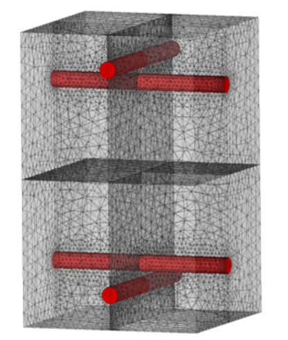
Fig. 265 Example of a unit RVE mesh for parameters identification (red: steel rebar, grey: concrete)#
An automated python ™ process generates automatically the RVE mesh from the following eleven geometrical parameters:
Plate thickness |
\(H\) |
|
|
Steel rebar spacing along \({x}_{1}\) and \({x}_{2}\) |
\(\mathrm{ex}\) and \(\mathrm{ey}\) |
|
Diameters of the four steel rebar |
|
|
\({x}_{3}\) positions of the four steel rebar |
This three-dimensional mesh includes the splitting of nodes located on steel-concrete interfaces (surfaces \({\Gamma}_{b}^{\zeta}\) ), the assignment of the different mesh zones to the sub-domains \({\Omega}_{i}^{1}\) , \({\Omega}_{i}^{2}\) , and periodicity of node locations for the external boundaries (normal unit vectors along \({x}_{1}\) and \({x}_{2}\) ). Microscopic material properties and boundary conditions prescribing, including periodicity in the RVE outer surfaces (upper and lower surfaces remaining free) and bond slip basis function are set.
Concerning the ten needed material parameters, the following table gathers the expected values:
2 elastic coefficients for steel |
Young’s modulus, Poisson’s ratio |
\({E}_{s}\) , \({\nu}_{s}\) |
2 elastic coefficients for concrete |
Young’s modulus, Poisson’s ratio |
\({E}_{c}\) , \({\nu}_{c}\) |
Usual engineering parameters for concrete |
Tensile and compressive strengths, maximal compressive strain, first compressive damage limit |
\({f}_{t}\) , \({f}_{c}\) , \({\epsilon}_{\mathrm{cm}}\) , \({f}_{\mathrm{dc}}\) |
Steel-concrete sliding experimental pull-out threshold parameter |
\({\tau}_{\mathrm{crit}}\) |
|
Post-peak tensile path parameter of local concrete constitutive relation |
\({\gamma}_{+}\) |
They are required in order to perform the \(342\) FEM elastic calculations on the RVE, see the table reported in the Appendix, at r7.01.37-auxiliary-problems-table, and DHRC threshold parameters determination.
The results of the numerical finite element simulations are used to identify the \(335\) DHRC macroscopic parameters with the help of a standard least square algorithm.
Remark 20:
In practice, if the obtained values of macroscopic coefficients of \({\mathbf{A}}^{\mathrm{mf}}(D)\) , \(\mathbf{C}(D)\) matrices are very small, and making consequently impossible the parameter identification, we decide to take the corresponding \(\alpha\) , \({\gamma}^{A}\) , \({\gamma}^{C}\) parameters equal to \(1\) and \({\gamma}^{B}\) parameters equal to \(0\) .
Analytical trivial example#
To illustrate the implementation of the previous approach, we take the following representative analytical trivial example.
The first step consists in verifying that the automatic procedure recovers the usual isotropic linear elastic plate stiffness tensor if we take, in the whole RVE, the same uniform sound elastic characteristics (\(E\) , \(\nu\) ). Indeed, in that case, the RVE \(\Omega\) is reduced to the simple segment \(]–H/2,H/2[\) along the axis \((O{e}_{({x}_{3})})\) ), and all the auxiliary fields \({\chi }^{\mathrm{\alpha \beta }}\) in membrane and \({\xi}^{\mathrm{\alpha \beta }}\) in bending depend only on \({x}_{3}\) . Solving in such situation the auxiliary problems (3–4), using first trial \(v({x}_{3})\) functions \(({v}_{1,}{v}_{2,}0)\) then \((0,0,{v}_{3})\) , we obtain easily:
Hence the macroscopic homogenised elastic plate tensor \(\mathbf{A}\) are:
Comparison of parameters with other constitutive models#
In order to give the user comparative information about DHRC parameters, with respect to other constitutive models, like GLRC_DM [r7.01.32], we propose the following evaluation in mono-axial loading cases, first in membrane, then in bending. The informations are calculated by the DHRC constitutive model automated identification procedure. So it is more easy to observe the influence of RVE material data on the DHRC parameters, before to perform the structural analysis itself..
Elastic coefficients#
We refer to the GLRC_DM model [r7.01.32], § 3.1, to express the RC equivalent elastic moduli in membrane (\({E}_{\mathrm{eq}}^{m}\) ) and in bending (\({E}_{\mathrm{eq}}^{f}\) ), from material data (concrete \({E}_{b}\) , \({\nu}_{b}\) and steel \({E}_{a}\) moduli) and geometrical data (steel section \({S}_{a}\) , thickness \(h\) , relative position of steel rebar in the thickness \({\chi }_{a}\in \left]0,1\right[\) ):
Therefore, the equivalent elastic RC plate coefficients in uniaxial membrane and in uniaxial bending can be deduced by:
According to the DHRC formulation in elastic domain, in particular tensor \({A}^{0}\) , we can express the membrane stress resultant in uniaxial loading case in terms of membrane uniaxial strain, in both \(x\) and \(y\) steel grids directions, and in the same way for the uniaxial bending case; we get then:
After elimination of all generalised strain variables except respectively \({\epsilon}_{xx}\) or \({\kappa}_{xx}\) , we easily derive the expressions of the equivalent elastic RC plate coefficients in uniaxial membrane and in uniaxial bending for the DHRC constitutive model, in the \(x\) steel grid direction, to be compared with the closed form GLRC_DM model ones:
To be more precise, the same calculations are also performed with the only mixture law contributions to tensor \({\mathbf{A}}^{0}\) , see r7.01.37-macroscopic-homogenised-model : this allows to observe the influence of auxiliary fields on final results.
We carry out the same calculations for the \(y\) steel grid direction.
Post-elastic coefficients#
In order to check the post-elastic response of the DHRC constitutive model, we calculable at the state \(D=0\) and \(\dot{D}>0\) the rate of stress resultants in radial monoaxial loading paths in respect of the rate of generalised strain variables, provided we have distinguished compressive then tensile cases for membrane loading. According to relations (4295) and (4296):
According to (3867), we recall that derivatives \({A}_{,D}(0)\) are directly dependent on tensor \({A}^{0}\) and \({\alpha}^{A}\) and \({\gamma}^{A}\) parameters, respectively in a tensile, compressive membrane, or positive or negative bending state. Moreover, the consistency conditions \({\dot{f}}_{({d}^{\rho})}=0\) give:
As we consider radial loading paths controlled by a regular \(h(t)\) function, we can write:
So we can write the rate equations in a concise manner:
where tensor \({A}^{T}\) results from contribution of \({A}^{0}\) and their derivatives at \(D=0\) , see equations (3879) and (3880) applied for the directions \(({E}_{1},{K}_{1})\) . And we apply to tensor \({A}^{T}\) the same procedure than done for tensor \({A}^{0}\) at r7.01.37-elastic-coefficients to calculate the equivalent post-elastic RC plate rate coefficients in uniaxial membrane (compressive then tensile cases) and in uniaxial bending for the DHRC constitutive model, in the \(x\) steel grid direction, then in \(y\) steel grid direction.
We refer to the GLRC_DM model [r7.01.32], § 3.2.2.1 and § 3.2.2.3, to express the RC equivalent post-elastic rate coefficients in membrane and in bending, I order to make comparison with DHRC constitutive model. We can also prefer to make this comparison with asymptotic slopes of membrane and bending responses of GLRC_DM model, see [r7.01.32], § 3.2.3.1 and § 3.2.3.3. Nevertheless, we can adopt the simplified expressions given in [r7.01.32], § 3.2.4.1 and § 3.2.4.3, involving \({\gamma}_{\mathrm{mt}}\) , \({\gamma}_{\mathrm{mc}}\) , \({\gamma}_{f}\) GLRC_DM parameters, acting as proportional reduction factors on elastic coefficients.
Internal variables of the DHRC model#
The internal variables output of Code_Aster are the following: the six fist are true thermodynamic internal variables, the five last ones are produced for easier post-treatment.
variables |
name |
contents |
\(\mathrm{V1}\) |
“ENDOSUP” |
\({D}_{1}\) Damage in the upper half of RVE |
\(\mathrm{V2}\) |
“ENDOINF” |
\({D}_{2}\) Damage in the lower half of RVE |
\(\mathrm{V3}\) |
“GLISXSUP” |
\({E}_{x}^{\eta 1}\) bond sliding of \(x\) rebar in the upper half of RVE |
\(\mathrm{V4}\) |
“GLISYSUP” |
\({E}_{y}^{\eta 1}\) bond sliding of \(y\) rebar in the upper half of RVE |
\(\mathrm{V5}\) |
“GLISXINF” |
\({E}_{x}^{\eta 2}\) bond sliding of \(x\) rebar in the lower half of RVE |
\(\mathrm{V6}\) |
“GLISYINF” |
\({E}_{y}^{\eta 2}\) bond sliding of \(y\) rebar in the lower half of RVE |
\(\mathrm{V7}\) |
“DISSENDO” |
Dissipated energy by damage: \({D}_{\mathrm{diss}}^{\mathrm{endo}}(t)={G}_{1}^{\mathrm{crit}}{D}_{1}(t)+{G}_{2}^{\mathrm{crit}}{D}_{2}(t)\) |
\(\mathrm{V8}\) |
“DISSGLIS” |
Dissipated energy by bond sliding: \(\begin{array}{}{D}_{\mathrm{diss}}^{\mathrm{bond}-\mathrm{slide}}(t)=\text{}\\ {\Sigma}_{x}^{\mathrm{crit}1}{\int}_{0}^{t}{\dot{E}}_{x}^{\eta 1}\mathrm{dt}+{\Sigma}_{y}^{\mathrm{crit}1}{\int}_{0}^{t}{\dot{E}}_{y}^{\eta 1}\mathrm{dt}+{\Sigma}_{x}^{\mathrm{crit}2}{\int}_{0}^{t}{\dot{E}}_{x}^{\eta 2}\mathrm{dt}+{\Sigma}_{y}^{\mathrm{crit}2}{\int}_{0}^{t}{\dot{E}}_{y}^{\eta 2}\mathrm{dt}\end{array}\) |
\(\mathrm{V9}\) |
“DISSIP” |
Sum of both energy dissipations |
\(\mathrm{V10}\) |
“ADOUMEMB” |
Mean relative weakening of membrane stiffness of reinforced concrete slab |
\(\mathrm{V11}\) |
“ADOUFLEX” |
Mean relative weakening of bending stiffness of reinforced concrete slab |
Distinction between upper and lower faces is made from the orientation of the local reference frame at each Gauss” point. So, the lower face is damaged \(\dot{{D}_{2}}>0\) for positive plate increasing curvatures, whereas the upper one is damaged \(\dot{{D}_{1}}>0\) for negative curvatures.
The \(\mathrm{V10}\) and \(\mathrm{V11}\) values are comparable to the equivalent scalar variables being produced by the GLRC_DM model, see [r7.01.32], to describe roughly the stiffness degradation of the RC plate. The respective calculated expressions are at each time-step:
They are being zero in absence of damage. These two variables neglect membrane-bending coupling.
Verification#
The model is verified by means of the test-cases: SSNS106C, H, I, J, L, M, N, O see [bib8], comparing with the GLRC_DM model results, whose parameters are identified in a consistent way and the ENDO_ISOT_BETON constitutive relation for the concrete and elastic rebar grids in a multi-layer RC plate modelling. The studied cases are:
ssns106 c |
Tensile-compressive with bending coupling loading cycle, low load level |
ssns106 i |
Pure bending alternate cyclic loading, high load level |
ssns106 j |
Tensile-compressive with bending coupling loading cycle, high load level |
ssns106 l |
Pure shear stress and shear strain alternate cyclic in plane loading, high load level |
snss106 m |
Pure shear stress and bending coupling alternate cyclic in plane loading, high load level |
ssns106 n |
Anticlastic bending alternate cyclic in plane loading, high load level |
ssns106 o |
Thermoelastic pure membrane loading cycle |
Post-elastic shear responses of the two DHRC and GLRC_DM models are significantly different. Indeed, the calibration done to align the two models in tension is no longer effective in shear strain stemming from the fact that DHRC shear strain behavior comes from the identification of the parameters by homogenization while with the GLRC_DM model this behavior is deduced from tensile and compressive responses working in the eigen-frame of the macroscopic membrane strains. Furthermore, the primary damage thresholds values GLRC_DM and DHRC are a little bit different. We can observe the significative contribution of sliding in the total dissipated energy obtained by the DHRC constitutive model, which is not get-at-able by the GLRC_DM one. Moreover, we observe that with model we get an increasing damage at each alternate cycle, which is not reproduced with the GLRC_DM one.
Validation#
The model is validated by means of comparison on some experimental data on reinforced concrete structures. The first one is an alternate compressive-tensile test on a reinforced concrete member, see test-cases: SSNS112, [bib18]. The second one considers a reinforced concrete beam under monotonic bending, see test-cases: SSNL119, [bib19]. The third one considers a reinforced concrete shear wall, under alternate increasing shear loading cycles, see test-cases: SSNS113, [bib20].
References#
Notice: the references to published materials quoted in the previous sections are available in [bib13].
[bib1] LEMAITRE J., CHABOCHE J.L.: «Mécanique des matériaux solides», Ed. Dunod (1985)
[bib2] P.Koechlin, S.Potapov. «A global constitutive model for reinforced concrete plates». ASCE J. Eng. Mech. 2006.
[bib3] P.Koechlin, S.Moulin. «Modèle de comportement global des plaques en béton armé sous chargement dynamique en flexion: loi GLRC améliorée: modélisation de la fissuration par endommagement». Note HT-62/02/021/A, 11/2002.
[bib4] F.VOLDOIRE. «Homogénéisation des structures hétérogènes». Note EDF/DER/MMN HI-74/93/055, 27/10/1993.
S.Moulin. «Modélisation des structures en béton armé sous chargement sismique». Note HT-62/04/025/A, 12/2004.
S.Moulin. F.VOLDOIRE «Étude d’une poutre en béton armé sous chargement de flexion». Note HT-62/05/013/A, 9/2006.
[bib7] J-J.MARIGO. «Étude numérique de l’endommagement». EDF, Bulletin des études et recherches, série C, n°2, pp.27-48, 1982.
[bib9] [r3.07.03] – Éléments de plaque DKT, DST, DKQ, DSQ et Q4G.
[bib10] [r7.01.04] – Loi de comportement ENDO_ISOT_BETON.
[bib11] [r7.01.32] – Loi de comportement GLRC_DM.
Ch.COMBESCURE; H.DUMONTET, F.VOLDOIRE. Homogenised constitutive model coupling damage and debonding for reinforced concrete structures under cyclic solicitations. Int. J. Sol. Struct., 50, pp. 3861–3874, 2013.
Ch.COMBESCURE; H.DUMONTET, F.VOLDOIRE. Dissipative Homogenised Reinforced Concrete (DHRC) constitutive model dedicated to reinforced concrete plates under seismic loading. Int. J. Sol. Struct., to be published, 2015.
[bib14] Ch.COMBESCURE. Formulation d’un modèle homogénéisé de plaque en béton armé pour des applications sismiques. Thèse de doctorat de l’université Pierre et Marie Curie, soutenue le 25 septembre 2013.
[bib15] P.SUQUET, 1982. Plasticité et homogénéisation. Thèse d’État, Université Paris VI.
F.VOLDOIRE, 1993. Homogénéisation des structures hétérogènes, Coll. Notes internes DER, ISSN 1161-059X, 1161-0611, Paris.
[v6.02.119] SSNL119 – Réponse statique d’une poutre en béton armé (section rectangulaire) à comportement non linéaire.
[v6.05.113] SSNS113 – Simulation de l’essai TESSH.
Appendix#
Auxiliary problems table#
We can find in the following table the sequence of \(342\) auxiliary problems calculation management, for membrane, bending and bond-sliding cases, for the different values of damage variables, used in the automated DHRC parameters identification procedure.
EPI value |
PRE_EPSI value |
Calculations number |
Membrane index |
Bending index |
Sliding index |
RVE |
Loading |
Damage |
Sliding |
Membrane aux. field |
Bending aux. field |
||||
-1 |
1 |
1 |
9 |
0 |
8 |
0 |
8 |
_ |
_ |
1X and 2X |
compression X |
yes |
no |
\({\chi }_{c}^{xx}\) |
\({\xi}_{c}^{xx}\) |
1 |
-1 |
10 |
18 |
9 |
17 |
9 |
17 |
_ |
_ |
1X and 2X |
tension X |
yes |
no |
\({\chi }_{t}^{xx}\) |
\({\xi}_{t}^{xx}\) |
-1 |
1 |
19 |
27 |
18 |
26 |
18 |
26 |
_ |
_ |
1X and 2X |
compression Y |
yes |
no |
\({\chi }_{c}^{yy}\) |
\({\xi}_{c}^{yy}\) |
1 |
-1 |
28 |
36 |
27 |
35 |
27 |
35 |
_ |
_ |
1X and 2X |
tension Y |
yes |
no |
\({\chi }_{t}^{yy}\) |
\({\xi}_{t}^{yy}\) |
0,5 |
-0,5 |
37 |
45 |
36 |
44 |
36 |
44 |
_ |
_ |
1X and 2X |
shear |
yes |
no |
\({\chi }^{xy}\) |
\({\xi}^{xy}\) |
-1 |
1 |
46 |
54 |
45 |
53 |
45 |
53 |
_ |
_ |
1Y and 2Y |
compression X |
yes |
no |
\({\chi }_{c}^{xx}\) |
\({\xi}_{c}^{xx}\) |
1 |
-1 |
55 |
63 |
54 |
62 |
54 |
62 |
_ |
_ |
1Y and 2Y |
tension X |
yes |
no |
\({\chi }_{t}^{xx}\) |
\({\xi}_{t}^{xx}\) |
-1 |
1 |
64 |
72 |
63 |
71 |
63 |
71 |
_ |
_ |
1Y and 2Y |
compression Y |
yes |
no |
\({\chi }_{c}^{yy}\) |
\({\xi}_{c}^{yy}\) |
1 |
-1 |
73 |
81 |
72 |
80 |
72 |
80 |
_ |
_ |
1Y and 2Y |
tension Y |
yes |
no |
\({\chi }_{t}^{yy}\) |
\({\xi}_{t}^{yy}\) |
0,5 |
-0,5 |
82 |
90 |
81 |
89 |
81 |
89 |
_ |
_ |
1Y and 2Y |
shear |
yes |
no |
\({\chi }^{xy}\) |
\({\xi}^{xy}\) |
-1 |
1 |
91 |
99 |
90 |
98 |
90 |
98 |
_ |
_ |
1T and 2T |
compression X |
yes |
no |
\({\chi }_{c}^{xx}\) |
\({\xi}_{c}^{xx}\) |
1 |
-1 |
100 |
108 |
99 |
107 |
99 |
107 |
_ |
_ |
1T and 2T |
tension X |
yes |
no |
\({\chi }_{t}^{xx}\) |
\({\xi}_{t}^{xx}\) |
-1 |
1 |
109 |
117 |
108 |
116 |
108 |
116 |
_ |
_ |
1T and 2T |
compression Y |
yes |
no |
\({\chi }_{c}^{yy}\) |
\({\xi}_{c}^{yy}\) |
1 |
-1 |
118 |
126 |
117 |
125 |
117 |
125 |
_ |
_ |
1T and 2T |
tension Y |
yes |
no |
\({\chi }_{t}^{yy}\) |
\({\xi}_{t}^{yy}\) |
0,5 |
-0,5 |
127 |
135 |
126 |
134 |
126 |
134 |
_ |
_ |
1T and 2T |
shear |
yes |
no |
\({\chi }^{xy}\) |
\({\xi}^{xy}\) |
0 |
0 |
136 |
144 |
135 |
143 |
_ |
_ |
0 |
8 |
1X and 2X |
_ |
no |
1X |
||
0 |
0 |
145 |
153 |
144 |
152 |
_ |
_ |
9 |
17 |
1X and 2X |
_ |
no |
2X |
||
0 |
0 |
154 |
162 |
153 |
161 |
_ |
_ |
18 |
26 |
1X and 2X |
_ |
no |
1Y |
||
0 |
0 |
163 |
171 |
162 |
170 |
_ |
_ |
27 |
35 |
1X and 2X |
_ |
no |
2Y |
||
0 |
0 |
172 |
180 |
171 |
179 |
_ |
_ |
36 |
44 |
1Y and 2Y |
_ |
no |
1X |
||
0 |
0 |
181 |
189 |
180 |
188 |
_ |
_ |
45 |
53 |
1Y and 2Y |
_ |
no |
2X |
||
0 |
0 |
190 |
198 |
189 |
197 |
_ |
_ |
54 |
62 |
1Y and 2Y |
_ |
no |
1Y |
||
0 |
0 |
199 |
207 |
198 |
206 |
_ |
_ |
63 |
71 |
1Y and 2Y |
_ |
no |
2Y |
||
Convexity of the strain energy density function with discontinuity in damage function#
As presented in section 3.1.2, the macroscopic free energy density \(W(E,K,{D}^{\zeta},{E}^{\eta \zeta })\) is continuous when its variables are taken in the whole strains and sliding strains space. However, the discontinuity in microscopic damage functions \(\xi (d)\) – due to the assumed distinction between tensile and compressive states, see Hyp 14 – induces a piece-wise definition of the elasticity tensors \({A}^{\mathrm{mm}}(D)\) and \({A}^{\mathrm{ff}}(D)\) , while \({A}^{\mathrm{mf}}(D)\) components don’t include this dissymmetry. We recall that, according to Remark 16, \(B(D)\) and \(C(D)\) tensors don’t entail any tension-compression dissymmetry. In domains sufficiently far from this discontinuity, it can be easily shown the convexity of the strain energy density function from its quadratic expression. Conversely, either side of this discontinuity, we have to proceed as proposed for instance by (Curnier, He, & Zysset, 1995).
As being assumed at Hyp 19, the discontinuity is defined by the hyperplane \(E+{Q}^{m\zeta }(D).{E}^{\eta \zeta }=0\) and \(K+{Q}^{f\zeta }(D).{E}^{\eta \zeta }=0\) , for \(D\) being fixed, with \({Q}^{\zeta}(D)={A}^{(-1)}(D):{B}^{\zeta}(D)\) defined by (4294).
We take profit that the stress resultants (4295) and (4296) obtained by derivation of the strain energy density function are continuous by construction with the discontinuity of \({A}^{\mathrm{mm}}(D)\) and \({A}^{\mathrm{ff}}(D)\) defined by the sign of \(x\) . Nevertheless, as we need to express the updated values of \({A}^{\mathrm{mm}}(D)\) and \({A}^{\mathrm{ff}}(D)\) components to determine \({Q}^{\zeta}(D)\) at each step increment, we decided to input the previous value \({D}^{-}\) , in an explicit algorithm way, see r7.01.37-finite-element-implementation .
Proof of the zero-valued tensor \(B\) if microscopic damage field is homogeneous in the RVE#
Let us recall that the tensor \(B\) components are defined by: \({B}_{\mathrm{\alpha \beta \gamma }}^{m\zeta }(D)={\langle \langle {a}_{\mathrm{\alpha \beta kl}}(d):{\epsilon}_{kl}({\chi }^{{\eta}_{\gamma}^{\zeta}})\rangle \rangle }_{\Omega}\) and \({B}_{\mathrm{\alpha \beta \gamma }}^{f\zeta }(D)={-\langle \langle {x}_{3}.{a}_{\mathrm{\alpha \beta kl}}(d):{\epsilon}_{kl}({\chi }^{{\eta}_{\gamma}^{\zeta}})\rangle \rangle }_{\Omega}\) , see (4291) and (4292). Let us assume that the components of the concrete damaged elastic tensor \({a}_{\mathrm{pqrs}}^{c}({d}^{\zeta})\) are symmetric with respect to the plane \({x}_{1}=0\) , i.e. \({\Gamma}_{s}\) see figure Fig. 262; moreover, according to the r7.01.37-non-uniform-steel-concrete-debonding , this tensor fulfils the symmetries with respect to the reference frame. Let us consider the auxiliary problem (4904) concerning the corrector \({\chi }^{{\eta}_{1}^{\zeta}}\) associated to sliding in the \({x}_{1}\) direction. Necessarily, we have the following properties: \({\chi }_{1}^{{\eta}_{1}^{\zeta}}\) is symmetric with respect to the plane \({x}_{1}=0\) , whereas \({\chi }_{2}^{{\eta}_{1}^{\zeta}}\) and \({\chi }_{3}^{{\eta}_{1}^{\zeta}}\) are antisymmetric. Therefore, \({a}_{\mathrm{iikl}}(d):{\epsilon}_{kl}({\chi }^{{\eta}_{1}^{\zeta}})\) and \({a}_{\mathrm{23kl}}(d):{\epsilon}_{kl}({\chi }^{{\eta}_{1}^{\zeta}})\) are antisymmetric with respect to the plane \({x}_{1}=0\) , whereas \({a}_{\mathrm{1jkl}}(d):{\epsilon}_{kl}({\chi }^{{\eta}_{1}^{\zeta}})\) are symmetric, for \(j\ne 1\) and \({a}_{\mathrm{1jkl}}(d):{\epsilon}_{kl}({\chi }^{{\eta}_{1}^{\zeta}})\) are antisymmetric with respect to the plane \({x}_{2}=0\) .
Performing the integration on the whole RVE, we deduce that: \({B}_{\mathrm{\alpha \beta 1}}^{m\zeta }(D)\) and \({B}_{\mathrm{\alpha \beta 1}}^{f\zeta }(D)\) vanish. The same reasoning holds for the other direction in the mid-plane of the RVE.
Since the tensor \(B\) manages the coupling between RC plate kinematics and steel bond sliding, we conclude that bond sliding can occur only if symmetry loss appears in the RVE, due to damage.